🙌 使用 FastFit 模型预测分析标注指标#
在本教程中,我们将使用 FastFit 库训练一个用于少样本分类的意图多分类器。然后,我们将进行一些预测并评估模型。最后,我们将使用 Argilla 模拟标注过程,并计算一些最知名的标注指标。
以下是我们将遵循的步骤
准备数据集
使用 FastFit 训练模型
进行预测并将其添加到 Argilla
评估标注性能
使用 argilla 计算准确率、精确率、召回率、F1 分数
使用 sklearn、seaborn 和 matplotlib 计算混淆矩阵
使用 argilla 计算 Krippendorff’s alpha
使用 sklearn 计算 Cohen’s kappa
使用 statsmodels 计算 Fleiss’ kappa
让我们开始吧!🚀
简介#
FastFit 是一个库,允许你使用少样本学习训练多分类器。它基于 transformers 库,并使用预训练模型在小型数据集上对其进行微调。当你的数据集很小并且想要快速训练模型时,这尤其有用。然而,SetFit 是另一个知名的库,它也允许使用 Sentence Transformers 进行少样本学习。
那么,为什么要使用一个而不是另一个呢?基于这篇 文章,作者比较了 FastFit、SetFit 和 Semantic Router,我们可以确定一些区别。
方面 |
FastFit |
SetFit |
|---|---|---|
准确率 |
高,但可能为了速度牺牲准确率 |
始终保持高水平 |
训练速度 |
快 |
慢 |
推理速度 |
慢 |
快 |
部署 |
容易,只需最少的专业知识 |
需要 transformers 知识 |
数据集处理 |
难以处理高度复杂的数据集 |
可以针对各种数据集进行微调 |
计算成本 |
较低 |
较高 |
在本教程中,我们将重点关注 FastFit,但你也可以尝试 SetFit 并比较结果。要了解如何使用 SetFit,你可以查看这篇 教程。
运行 Argilla#
对于本教程,你将需要运行 Argilla 服务器。部署和运行 Argilla 主要有两种选择
在 Hugging Face Spaces 上部署 Argilla:如果你想使用外部 Notebook(例如,Google Colab)运行教程,并且你拥有 Hugging Face 帐户,则只需点击几下即可在 Spaces 上部署 Argilla

有关配置部署的详细信息,请查看 官方 Hugging Face Hub 指南。
使用 Argilla 的快速入门 Docker 镜像启动 Argilla:如果你想在 本地计算机上运行 Argilla,这是推荐的选项。请注意,此选项仅允许你在本地运行教程,而不能与外部 Notebook 服务一起运行。
有关部署选项的更多信息,请查看文档的部署部分。
提示
本教程是一个 Jupyter Notebook。有两种运行它的选项
使用此页面顶部的“在 Colab 中打开”按钮。此选项允许你直接在 Google Colab 上运行 Notebook。不要忘记将运行时类型更改为 GPU 以加快模型训练和推理速度。
通过单击页面顶部的“查看源码”链接下载 .ipynb 文件。此选项允许你下载 Notebook 并在本地计算机或你选择的 Jupyter Notebook 工具上运行它。
设置环境#
要完成本教程,你将需要使用 pip 安装 Argilla 客户端和一些第三方库
[ ]:
!pip install argilla fast-fit datasets
!pip install nltk statsmodels seaborn matplotlib
让我们进行必要的导入
[ ]:
import random

import matplotlib.pyplot as plt
import numpy as np
import seaborn as sns
from sklearn.metrics import cohen_kappa_score, confusion_matrix
from statsmodels.stats.inter_rater import fleiss_kappa

from datasets import Dataset, DatasetDict, load_dataset
from transformers import AutoTokenizer, pipeline

import argilla as rg
from argilla.client.feedback.metrics import ModelMetric, AgreementMetric

from fastfit import FastFit, FastFitTrainer, sample_dataset
如果你使用 Docker 快速入门镜像或公共 Hugging Face Spaces 运行 Argilla,则需要使用 URL 和 API_KEY 初始化 Argilla 客户端
[ ]:
# Replace api_url with the url to your HF Spaces URL if using Spaces
# Replace api_key if you configured a custom API key
# Replace workspace with the name of your workspace
rg.init(
    api_url="https://:6900",
    api_key="owner.apikey",
    workspace="admin"
)
如果你运行的是私有 Hugging Face Space,你还需要按如下方式设置 HF_TOKEN
[ ]:
# # Set the HF_TOKEN environment variable
# import os
# os.environ['HF_TOKEN'] = "your-hf-token"

# # Replace api_url with the url to your HF Spaces URL
# # Replace api_key if you configured a custom API key
# rg.init(
#     api_url="https://[your-owner-name]-[your_space_name].hf.space",
#     api_key="admin.apikey",
#     extra_headers={"Authorization": f"Bearer {os.environ['HF_TOKEN']}"},
# )
启用遥测#
我们从你与教程的互动中获得宝贵的见解。为了改进自身,以便为你提供最合适的内容,使用以下代码行将帮助我们了解本教程是否有效地为你服务。虽然这是完全匿名的,但如果你愿意,可以选择跳过此步骤。有关更多信息,请查看 遥测 页面。
[ ]:
try:
    from argilla.utils.telemetry import tutorial_running
    tutorial_running()
except ImportError:
    print("Telemetry is introduced in Argilla 1.20.0 and not found in the current installation. Skipping telemetry.")
准备数据集#
首先,我们将准备数据集来训练意图分类器,该分类器负责使用预定义的意图准确标记自然语言话语。FastFit 对于少样本多分类特别有效,尤其是在具有许多语义相似类别的场景中。因此,我们选择使用 Hugging Face 的 contemmcm/clinc150 数据集。此数据集包含 151 个意图类别,非常适合我们的需求。
[55]:
# Load the dataset
hf_dataset = load_dataset("contemmcm/clinc150", split="complete")
hf_dataset
[55]:
Dataset({
    features: ['text', 'domain', 'intent', 'split'],
    num_rows: 23700
})
[56]:
# Get the 151 classes and prepare the conversion dictionaries
labels = [label for label in hf_dataset.features["intent"].names if label]
label2id = {label:id for id, label in enumerate(labels)}
id2label = {id:label for label, id in label2id.items()}
len(labels)
[56]:
151
数据集没有预定义的划分,因此我们将根据 split 列对其进行拆分,仅选择 train、validation 和 test 拆分。我们将仅保留 text 和 intent 列,并将意图 ID 转换为标签。
[57]:
# Save the needed data
splits = ['train', 'val', 'test']

data = {split: {'text': [], 'intent': []} for split in splits}

for split in splits:
    for entry in hf_dataset:
        if entry['split'] == split:
            data[split]['text'].append(entry['text'])
            data[split]['intent'].append(id2label[entry['intent']])

# Create the dataset
dataset = DatasetDict({split: Dataset.from_dict(data[split]) for split in data})
由于这是少样本学习,我们不需要使用训练集中的所有示例。因此,我们将使用 FastFit 的 sample_dataset 方法来为每个类别选择 10 个示例(由于 FastFit 训练速度更快,我们可以承担包含更多样本的风险,而无需担心训练时间显着增加)。此外,我们将重命名 val 拆分为 validation 以符合 FastFit 要求。
[60]:
# Sample the dataset
dataset["train"] = sample_dataset(dataset["train"], label_column="intent", num_samples_per_label=10, seed=42)

# Rename the validation split
dataset['validation'] = dataset.pop('val')

dataset
[60]:
DatasetDict({
    train: Dataset({
        features: ['text', 'intent'],
        num_rows: 1500
    })
    test: Dataset({
        features: ['text', 'intent'],
        num_rows: 4500
    })
    validation: Dataset({
        features: ['text', 'intent'],
        num_rows: 3000
    })
})
使用 FastFit 训练#
正如我们所提到的,FastFit 是一个用于少样本学习的库,可用于使用每个类别的一些示例来训练模型。此外,他们创建了用于多分类的 FewMany 基准。
在本例中,我们选择使用 sentence-transformers/paraphrase-mpnet-base-v2 模型来训练意图分类器,因为其大小和性能。但是,你可以探索 Hugging Face 上提供的其他模型,并通过查阅 MTEB 排行榜 找到最合适的模型。FastFitTrainer 中设置的大多数参数都是默认值,但你可以根据需要更改它们。
[ ]:
# Initialize the FastFitTrainer
trainer = FastFitTrainer(
    model_name_or_path="sentence-transformers/paraphrase-mpnet-base-v2",
    label_column_name="intent",
    text_column_name="text",
    num_train_epochs=25,
    per_device_train_batch_size=32,
    per_device_eval_batch_size=64,
    max_text_length=128,
    dataloader_drop_last=False,
    num_repeats=4,
    optim="adafactor",
    clf_loss_factor=0.1,
    fp16=True,
    dataset=dataset,
)
[232]:
# Train the model
model = trainer.train()
| 步骤 | 训练损失 |
|---|---|
| 500 | 2.676200 |
| 1000 | 2.590300 |
***** train metrics *****
  epoch                    =       25.0
  total_flos               =        0GF
  train_loss               =     2.6261
  train_runtime            = 0:02:59.32
  train_samples            =       1500
  train_samples_per_second =    209.121
  train_steps_per_second   =      6.552
正如我们所见,训练时间仅用了 3 分钟,这非常快。现在,让我们评估模型以检查其准确率。评估后,我们将模型保存到磁盘以进行推理步骤。
[234]:
# Evaluate the model
results = trainer.evaluate()
***** eval metrics *****
  epoch                   =       25.0
  eval_accuracy           =      0.947
  eval_loss               =     2.9615
  eval_runtime            = 0:00:04.30
  eval_samples            =       3000
  eval_samples_per_second =    697.334
  eval_steps_per_second   =     10.925
[236]:
# Save the model
model.save_pretrained("intent_fastfit_model")
使用我们的模型进行推理#
正如我们所见,看起来我们有一个模型已准备好进行预测。让我们加载模型和 tokenizer。
[52]:
# Load the model and tokenizer
model = FastFit.from_pretrained("intent_fastfit_model")
tokenizer = AutoTokenizer.from_pretrained("sentence-transformers/paraphrase-mpnet-base-v2")
接下来,我们将准备我们的 pipeline。
初始化 pipeline 时会引发错误警告:
The model 'FastFit' is not supported for text-classification。但是,分类器将正常工作。
如果你更改了基础模型,则可能会遇到
token_type_ids错误。你可以按照 此处 注明的方式解决它。
我们将 top_k=1 设置为获取每个预测的最有可能的类别。如果你想获取所有预测类别,请将其设置为 None。
[ ]:
# Define the pipeline
classifier = pipeline("text-classification", model=model, tokenizer=tokenizer, top_k=1)
那么,让我们进行一些预测!为了本教程的目的,我们将使用验证拆分,并且仅使用前 100 个样本。正如我们在初始运行时观察到的,进行预测花费了一分钟以上。因此,正如引言中所述,如果我们需要进行更多预测,那将会很慢。
[61]:
# Make predictions
predictions = [
    {
        "text": sample["text"],
        "true_intent": sample["intent"],
        "predicted_intent": classifier(sample["text"])
    }
    for sample in dataset['validation'].to_list()[:100]
]
[62]:
for p in predictions[:5]:
    print(p)
{'text': "what's the weather today", 'true_intent': 'utility:weather', 'predicted_intent': [[{'label': 'utility:weather', 'score': 0.8783325552940369}]]}
{'text': 'what are the steps required for making a vacation request', 'true_intent': 'work:pto_request', 'predicted_intent': [[{'label': 'work:pto_request', 'score': 0.9850018620491028}]]}
{'text': 'help me set a timer please', 'true_intent': 'utility:timer', 'predicted_intent': [[{'label': 'utility:timer', 'score': 0.8667100071907043}]]}
{'text': 'what is the mpg for this car', 'true_intent': 'auto_and_commute:mpg', 'predicted_intent': [[{'label': 'auto_and_commute:mpg', 'score': 0.9732610583305359}]]}
{'text': 'was my last transaction at walmart', 'true_intent': 'banking:transactions', 'predicted_intent': [[{'label': 'banking:transactions', 'score': 0.9001362919807434}]]}
使用 Argilla 标注#
我们将使用 Argilla 模拟标注过程。首先,我们需要创建一个数据集。我们将使用预定义的文本分类任务模板,仅指定要标注的标签。
有关任务模板的更详细说明或自定义数据集,请查看 Argilla 文档。
[25]:
# Define the feedback dataset
dataset = rg.FeedbackDataset.for_text_classification(
    labels=labels,
)
dataset
[25]:
FeedbackDataset(
   fields=[TextField(name='text', title='Text', required=True, type='text', use_markdown=False)]
   questions=[LabelQuestion(name='label', title='Label', description='Classify the text by selecting the correct label from the given list of labels.', required=True, type='label_selection', labels=['oos:oos', 'banking:freeze_account', 'banking:routing', 'banking:pin_change', 'banking:bill_due', 'banking:pay_bill', 'banking:account_blocked', 'banking:interest_rate', 'banking:min_payment', 'banking:bill_balance', 'banking:transfer', 'banking:order_checks', 'banking:balance', 'banking:spending_history', 'banking:transactions', 'banking:report_fraud', 'credit_cards:replacement_card_duration', 'credit_cards:expiration_date', 'credit_cards:damaged_card', 'credit_cards:improve_credit_score', 'credit_cards:report_lost_card', 'credit_cards:card_declined', 'credit_cards:credit_limit_change', 'credit_cards:apr', 'credit_cards:redeem_rewards', 'credit_cards:credit_limit', 'credit_cards:rewards_balance', 'credit_cards:application_status', 'credit_cards:credit_score', 'credit_cards:new_card', 'credit_cards:international_fees', 'kitchen_and_dining:food_last', 'kitchen_and_dining:confirm_reservation', 'kitchen_and_dining:how_busy', 'kitchen_and_dining:ingredients_list', 'kitchen_and_dining:calories', 'kitchen_and_dining:nutrition_info', 'kitchen_and_dining:recipe', 'kitchen_and_dining:restaurant_reviews', 'kitchen_and_dining:restaurant_reservation', 'kitchen_and_dining:meal_suggestion', 'kitchen_and_dining:restaurant_suggestion', 'kitchen_and_dining:cancel_reservation', 'kitchen_and_dining:ingredient_substitution', 'kitchen_and_dining:cook_time', 'kitchen_and_dining:accept_reservations', 'home:what_song', 'home:play_music', 'home:todo_list_update', 'home:reminder', 'home:reminder_update', 'home:calendar_update', 'home:order_status', 'home:update_playlist', 'home:shopping_list', 'home:calendar', 'home:next_song', 'home:order', 'home:todo_list', 'home:shopping_list_update', 'home:smart_home', 'auto_and_commute:current_location', 'auto_and_commute:oil_change_when', 'auto_and_commute:oil_change_how', 'auto_and_commute:uber', 'auto_and_commute:traffic', 'auto_and_commute:tire_pressure', 'auto_and_commute:schedule_maintenance', 'auto_and_commute:gas', 'auto_and_commute:mpg', 'auto_and_commute:distance', 'auto_and_commute:directions', 'auto_and_commute:last_maintenance', 'auto_and_commute:gas_type', 'auto_and_commute:tire_change', 'auto_and_commute:jump_start', 'travel:plug_type', 'travel:travel_notification', 'travel:translate', 'travel:flight_status', 'travel:international_visa', 'travel:timezone', 'travel:exchange_rate', 'travel:travel_suggestion', 'travel:travel_alert', 'travel:vaccines', 'travel:lost_luggage', 'travel:book_flight', 'travel:book_hotel', 'travel:carry_on', 'travel:car_rental', 'utility:weather', 'utility:alarm', 'utility:date', 'utility:find_phone', 'utility:share_location', 'utility:timer', 'utility:make_call', 'utility:calculator', 'utility:definition', 'utility:measurement_conversion', 'utility:flip_coin', 'utility:spelling', 'utility:time', 'utility:roll_dice', 'utility:text', 'work:pto_request_status', 'work:next_holiday', 'work:insurance_change', 'work:insurance', 'work:meeting_schedule', 'work:payday', 'work:taxes', 'work:income', 'work:rollover_401k', 'work:pto_balance', 'work:pto_request', 'work:w2', 'work:schedule_meeting', 'work:direct_deposit', 'work:pto_used', 'small_talk:who_made_you', 'small_talk:meaning_of_life', 'small_talk:who_do_you_work_for', 'small_talk:do_you_have_pets', 'small_talk:what_are_your_hobbies', 'small_talk:fun_fact', 'small_talk:what_is_your_name', 'small_talk:where_are_you_from', 'small_talk:goodbye', 'small_talk:thank_you', 'small_talk:greeting', 'small_talk:tell_joke', 'small_talk:are_you_a_bot', 'small_talk:how_old_are_you', 'small_talk:what_can_i_ask_you', 'meta:change_speed', 'meta:user_name', 'meta:whisper_mode', 'meta:yes', 'meta:change_volume', 'meta:no', 'meta:change_language', 'meta:repeat', 'meta:change_accent', 'meta:cancel', 'meta:sync_device', 'meta:change_user_name', 'meta:change_ai_name', 'meta:reset_settings', 'meta:maybe'], visible_labels=20)]
   guidelines=This is a text classification dataset that contains texts and labels. Given a set of texts and a predefined set of labels, the goal of text classification is to assign one label to each text based on its content. Please classify the texts by making the correct selection.)
   metadata_properties=[])
   vectors_settings=[])
)
标准标注过程包括将记录添加到数据集,其中包含要标注的文本和预测标签以及其分数作为建议,以帮助标注员。但是,对于本教程并模拟标注过程,我们还将添加响应。具体来说,我们将为每个记录添加三个响应:一个带有正确标签,一个带有随机标签(正确标签或不同标签),以及一个带有预测标签。
要了解如何创建用户,请查看 Argilla 文档。
[26]:
# Get the list of users
users = rg.User.list()

# Define the feedback records
records = [
    rg.FeedbackRecord(
        fields={
            "text": sample["text"],
        },
        suggestions=[
            {
                "question_name": "label",
                "value": sample["predicted_intent"][0][0]["label"],
                "score": round(sample["predicted_intent"][0][0]["score"], 2),
            }
        ],
        responses=[
            {
                "values": {
                    "label": {
                        "value": sample["true_intent"],
                    }
                },
                "user_id": users[0].id
            },
            {
                "values": {
                    "label": {
                        "value": random.choice([sample["true_intent"], labels[0]]),
                    }
                },
                "user_id": users[1].id
            },
            {
                "values": {
                    "label": {
                        "value": sample["predicted_intent"][0][0]["label"],
                    }
                },
                "user_id": users[2].id
            }
        ]
    ) for sample in predictions
]
dataset.add_records(records)
我们可以将数据集推送到 Argilla 以在 UI 中可视化。
[ ]:
dataset.push_to_argilla(name="intent_feedback_dataset", workspace="admin")

分析标注性能#
一旦我们的数据集被标注,我们就可以通过不同的方式分析标注性能。首先,我们需要检索标注的数据集并保存所需的信息以计算指标。
[40]:
# Retrieve the annotated dataset
feedback_dataset = rg.FeedbackDataset.from_argilla(name="intent_feedback_dataset", workspace="admin")
[ ]:
# Save the list of responses by annotator
responses_by_annotator = {}
for record in feedback_dataset.records:
    if record.responses:
        submitted_responses = [response for response in record.responses if response.status == "submitted"]
        for response in submitted_responses:
            print(response)
            annotator_id = str(response.user_id)
            if annotator_id not in responses_by_annotator:
                responses_by_annotator[annotator_id] = []
            responses_by_annotator[annotator_id].append(response.values["label"].value)
[ ]:
# You can check the responses directly using the id of the annotator
responses_by_annotator[str(users[0].id)]

# or the name of the annotator
responses_by_annotator[str(rg.User.from_name("argilla").id)]
准确率、精确率、召回率和 F1 分数#
Argilla 允许你计算标注数据集的准确率、精确率、召回率和 F1 分数。它将比较建议的标签与标注的标签,并计算每个记录和整个数据集的指标。
有关指标的更多信息,请查看 Argilla 文档。
[ ]:
# List of metrics to compute
metrics = ["accuracy", "precision", "recall", "f1-score"]

# Initialize the ModelMetric object
metric = ModelMetric(dataset=feedback_dataset, question_name="label")

# Save the metrics per annotator
annotator_metrics = {}
for metric_name in metrics:
    annotator_metrics[metric_name] = metric.compute(metric_name)
此设置使我们能够观察到一位具有完美准确率的标注员和另一位具有中等水平性能的标注员。鉴于建议是预测并且其可靠性不确定,此模拟有助于我们评估标注员是否受到建议的影响,或者他们是否正在独立地准确标注。这样,我们可以更好地了解建议对标注质量的影响。
[43]:
annotator_metrics["accuracy"]
[43]:
{'e106d194-10b6-4608-a2e9-aea40cfd90d0': [ModelMetricResult(metric_name='accuracy', count=100, result=0.92)],
 '0bcc381d-0c77-4ef8-8de0-83417fd5a80b': [ModelMetricResult(metric_name='accuracy', count=100, result=0.45)],
 '13f90c69-1cb8-42c2-a861-491f25878ff3': [ModelMetricResult(metric_name='accuracy', count=100, result=1.0)]}
混淆矩阵#
理解标注性能的一个有用工具是可视化混淆矩阵。它显示了每个类别的正确和不正确标注的数量,使我们能够识别哪些类别对标注员来说更具挑战性。你可以使用 sklearn 的 confusion_matrix 函数计算它,并使用 seaborn 和 matplotlib 绘制它。
[ ]:
# Compute the confusion matrix for annotator 2 (his responses were the predicted labels)
true_labels = responses_by_annotator[str(users[2].id)]
predicted_labels = [sample["predicted_intent"][0][0]["label"] for sample in predictions]

confusion_matrix = confusion_matrix(true_labels, predicted_labels)
[ ]:
# Create a heatmap with seaborn and matplotlib
plt.figure(figsize=(7, 5))
sns.heatmap(confusion_matrix, annot=False, fmt='d', cmap='Blues')
plt.xlabel('Predicted')
plt.ylabel('True')
plt.title('Confusion Matrix')
plt.show()

# plt.savefig('confusion_matrix.png', dpi=300) # save the image
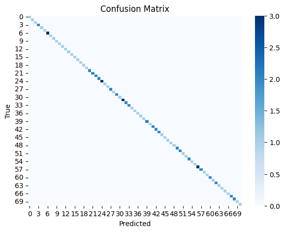
在上图中,对角线表示正确的标注,其中颜色强度表示标注的数量。非对角线元素表示不正确的标注,它们也用颜色编码,但在这种情况下,标注员 2 的标注看起来与真实标签匹配。请注意,标签的数量低于 151,因为我们使用的是验证拆分的子集。
Krippendorff’s Alpha#
对于标注员间一致性,Argilla 允许你计算 Krippendorff’s alpha。此指标广泛用于标注领域,用于衡量两个或多个标注员之间的一致性,并被认为是最可靠的指标之一。它的范围从 0 到 1,其中 0 表示没有一致性,1 表示完全一致。
有关指标的更多信息,请查看 Argilla 文档。
[ ]:
# Compute Krippendorff's Alpha
metric = AgreementMetric(dataset=feedback_dataset, question_name="label")
agreement_metric = metric.compute("alpha")
我们看到标注员之间的中等水平一致性,这是预期的,因为标注员 1 提供了随机响应。
[3]:
agreement_metric
[3]:
AgreementMetricResult(metric_name='alpha', count=300, result=0.6131595970797523)
Cohen’s Kappa#
Coher’s kappa 是另一个用于衡量一致性的指标,但仅限于两个标注员标注相同数据的情况。它考虑了偶然达成一致的可能性。它的范围从 -1 到 1,其中 1 表示完全一致,0 表示没有一致性,-1 表示完全不一致。我们可以使用 sklearn 的 cohen_kappa_score 函数计算它。
[49]:
# Compute Cohen's Kappa for each pair of annotators
annotator1_2 = cohen_kappa_score(responses_by_annotator[str(users[0].id)], responses_by_annotator[str(users[1].id)])
annotator2_3 = cohen_kappa_score(responses_by_annotator[str(users[1].id)], responses_by_annotator[str(users[2].id)])
annotator1_3 = cohen_kappa_score(responses_by_annotator[str(users[0].id)], responses_by_annotator[str(users[2].id)])
[51]:
print(f"Cohen's Kappa between annotator 1 and 2: {annotator1_2}")
print(f"Cohen's Kappa between annotator 2 and 3: {annotator2_3}")
print(f"Cohen's Kappa between annotator 1 and 3: {annotator1_3}")
Cohen's Kappa between annotator 1 and 2: 0.5059985885673959
Cohen's Kappa between annotator 2 and 3: 0.44567627494456763
Cohen's Kappa between annotator 1 and 3: 0.9187074484300376
我们观察到标注员 1(基于真实标签的响应)和 3(基于预测标签的响应)之间的高度一致性。然而,与标注员 2 的一致性较低,因为其答案是随机的。
Fleiss’ Kappa#
Fleiss’ kappa 与 Cohen’s kappa 类似,但允许超过两个标注员。同样,它的范围从 -1 到 1,其中 1 表示完全一致,0 表示没有一致性,-1 表示完全不一致。我们可以使用 statsmodels 中的 fleiss_kappa 函数计算它。
[81]:
# Initialize ratings matrix with the number of records and labels
ratings = np.zeros((100, 151))

# Populate the matrix
for annotator, responses in responses_by_annotator.items():
    for i, response in enumerate(responses):
        ratings[i, label2id[response]] += 1

# Compute Fleiss' Kappa
kappa = fleiss_kappa(ratings, method='fleiss')
我们可以看到,一致性与 Krippendorff’s alpha 相似,后者也评估了两个以上的标注员。
[85]:
print("Fleiss' Kappa:", kappa)
Fleiss' Kappa: 0.611865816467979
结论#
在本教程中,我们使用 FastFit 训练了一个意图分类器,进行了预测,并使用 Argilla 模拟了标注过程。标注员 1 的响应基于真实标签,标注员 2 在真实标签和不正确标签之间交替,标注员 3 的响应基于预测标签。然后,我们计算了标注指标,包括准确率、精确率、召回率、F1 分数、Krippendorff’s alpha、Cohen’s kappa 和 Fleiss’ kappa。我们还可视化了混淆矩阵,以更好地理解标注性能。这些指标展示了标注员 1 和 3 的出色表现和一致性,而由于标注员 2 的响应,总体一致性为中等水平。