🥇 比较文本分类模型#
在本教程中,您将学习如何使用两个不同的模型对数据集进行文本分类,将模型预测上传到您的 Argilla 工作区,并通过计算每个模型的 F1 分数来比较模型。它将引导您完成以下步骤: - 💾 加载您想要使用的数据集。 - 💻 使用零样本分类模型计算预测。 - 🔄 将模型输出转换为 Argilla 格式并上传到 Argilla 工作区。 - 💻 使用零样本 SetFit 模型计算预测。 - 🧪 使用 F1 分数比较模型预测
简介#
在进行文本分类工作时,您可能想要比较两个模型以决定使用哪个模型。为此,我们使用模型的注释作为真实文本类别,计算训练模型的 F1 分数。F1 分数可以解释为精确率和召回率的调和平均值,其中 F1 分数的最佳值为 1,最差值为 0。(更多信息请参考此文档)
Argilla 允许您部署和监控您喜欢的任何模型,但在本教程中,我们将重点关注 NLP 领域中最常用的两个框架:transformers 和 SetFit。让我们开始吧!
运行 Argilla#
对于本教程,您需要运行 Argilla 服务器。部署和运行 Argilla 有两个主要选项
在 Hugging Face Spaces 上部署 Argilla:如果您想使用外部笔记本(例如,Google Colab)运行教程,并且您在 Hugging Face 上有帐户,则只需点击几下即可在 Spaces 上部署 Argilla

有关配置部署的详细信息,请查看官方 Hugging Face Hub 指南。
使用 Argilla 的快速入门 Docker 镜像启动 Argilla:如果您想在本地机器上运行 Argilla,这是推荐的选项。请注意,此选项仅允许您在本地运行教程,而不能与外部笔记本服务一起运行。
有关部署选项的更多信息,请查看文档的部署部分。
提示
本教程是一个 Jupyter Notebook。有两种运行方式
使用此页面顶部的“在 Colab 中打开”按钮。此选项允许您直接在 Google Colab 上运行 notebook。不要忘记将运行时类型更改为 GPU 以加快模型训练和推理速度。
单击页面顶部的“查看源代码”链接下载 .ipynb 文件。此选项允许您下载 notebook 并在本地机器或您选择的 Jupyter Notebook 工具上运行它。
设置#
要完成本教程,您需要使用 pip 安装 Argilla 客户端和一些第三方库
[1]:
%pip install transformers argilla datasets torch setfit -qqqqqqq
所需的导入
[2]:
import argilla as rg
from datasets import load_dataset
from transformers import pipeline
from argilla.metrics.text_classification import f1
import pandas as pd
如果您正在使用 Docker 快速入门镜像或 Hugging Face Spaces 运行 Argilla,您需要使用 URL 和 API_KEY 初始化 Argilla 客户端
[3]:
# Replace api_url with the url to your HF Spaces URL if using Spaces
# Replace api_key if you configured a custom API key
# Replace workspace with the name of your workspace
rg.init(
    api_url="https://:6900",
    api_key="owner.apikey",
    workspace="admin"
)
如果您正在运行私有的 Hugging Face Space,您还需要设置 HF_TOKEN,如下所示
[ ]:
# # Set the HF_TOKEN environment variable
# import os
# os.environ['HF_TOKEN'] = "your-hf-token"

# # Replace api_url with the url to your HF Spaces URL
# # Replace api_key if you configured a custom API key
# # Replace workspace with the name of your workspace
# rg.init(
#     api_url="https://[your-owner-name]-[your_space_name].hf.space",
#     api_key="owner.apikey",
#     workspace="admin",
#     extra_headers={"Authorization": f"Bearer {os.environ['HF_TOKEN']}"},
# )
本教程选择 HugginFace ag_news 数据集
[ ]:
news_dataset = load_dataset("ag_news", split="test")
此数据集由两列组成,一列是新闻文章的文本,另一列是与该文本文章关联的标签
对于本教程,我们将标签视为文本的注释
我们转换数据集以创建一个 argilla TextClassificationDataset
[ ]:
int_to_label = {
    0:"World",
    1:"Sports",
    2:"Business",
    3:"Sci/Tech",
}

news_dataset = news_dataset.map(lambda row: {"prediction": [{"label":int_to_label[row["label"]], "score":1}]})
[ ]:
ds_record = rg.read_datasets(dataset=news_dataset, task="TextClassification")
启用遥测#
我们从您与我们教程的互动中获得宝贵的见解。为了改进我们自己,为您提供最合适的内容,使用以下代码行将帮助我们了解本教程是否有效地为您服务。虽然这是完全匿名的,但如果您愿意,可以选择跳过此步骤。有关更多信息,请查看遥测页面。
[ ]:
try:
    from argilla.utils.telemetry import tutorial_running
    tutorial_running()
except ImportError:
    print("Telemetry is introduced in Argilla 1.20.0 and not found in the current installation. Skipping telemetry.")
使用 transformers 进行零样本文本分类预测#
在 HugginFace 上,我们选择模型 cross-encoder/nli-distilroberta-base,该模型经过训练以执行零样本分类。我们使用此模型创建一个 pipeline,然后执行预测。
注意:``pipeline()`` 中的 ``device=0`` 允许使用 GPU,如果您没有可用的 GPU,请删除此参数
[7]:
labels =["Sports", "Sci/Tech", "Business", "World"]

pipe = pipeline("zero-shot-classification", model='cross-encoder/nli-distilroberta-base', device=0)
result = []
with pipe.device_placement():
  result = pipe(
    [data.text for data in ds_record],
    candidate_labels=labels,
  )
现在已经使用零样本模型成功进行了预测,我们可以将其转换为 argilla TextClassificationRecord 列表并上传到我们的 argilla 客户端
[ ]:
zero_shot_news_dataset = [
rg.TextClassificationRecord(
text=res["sequence"],
prediction=list(zip(res['labels'],res['scores'])),
annotation=record.prediction[0][0],
) for res, record in zip(result, ds_record)
]
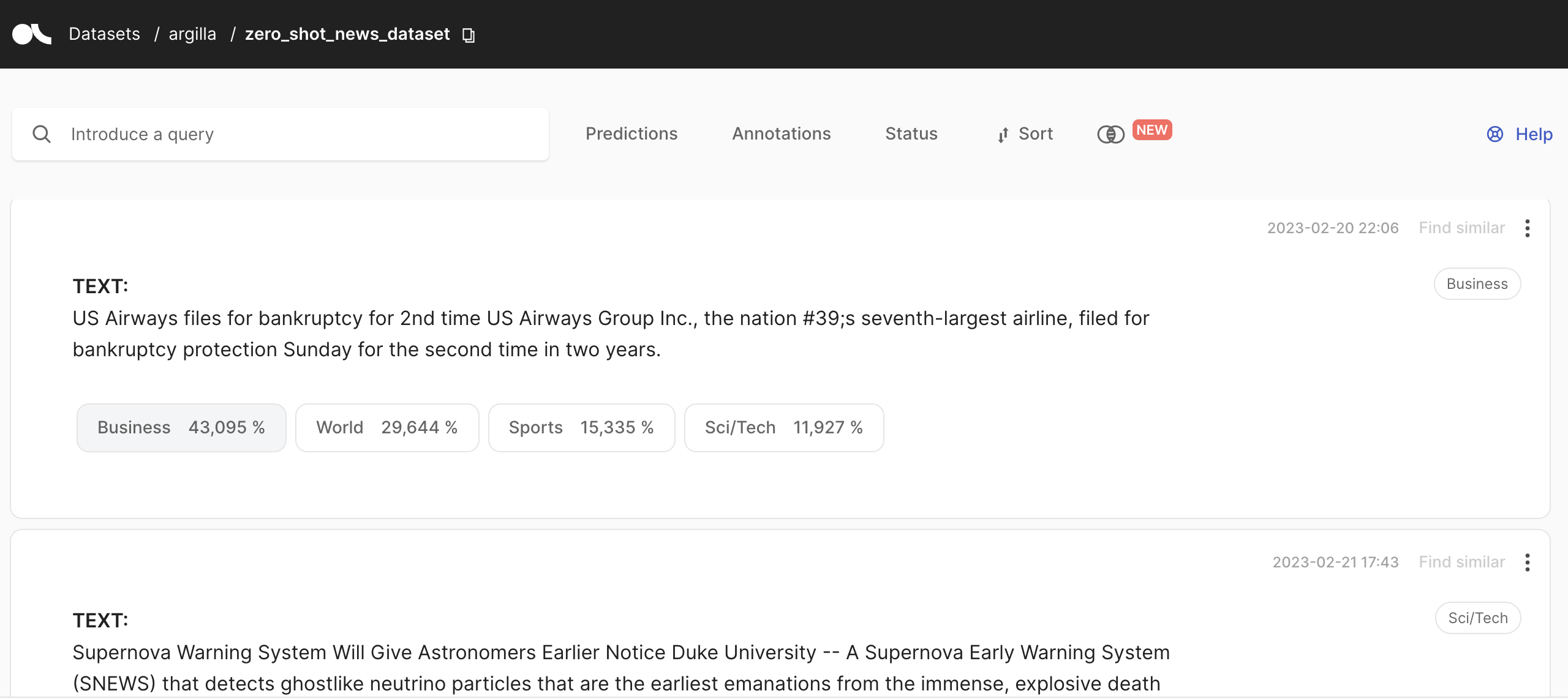
rg.log(name="zero_shot_news_dataset", records=zero_shot_news_dataset)
您可以在 Argilla UI 中访问 zero_shot_news_dataset
最后,我们使用 argilla f1 函数测量模型的性能,该函数计算 F1 分数
[9]:
f1_zero_shot = f1("zero_shot_news_dataset")
f1_zero_shot.visualize()
使用训练好的 SetFit 分类器进行零样本文本分类#
所需的导入
[10]:
from setfit import SetFitModel, SetFitTrainer, get_templated_dataset
我们使用数据集的标签创建训练示例的合成数据集
[11]:
labels = ["Sports", "Sci/Tech", "Business", "World"]
train_dataset = get_templated_dataset(
    candidate_labels=labels,
    sample_size=8,
    template="The news article is about {}"
)
我们使用预训练模型 ‘all-MiniLM-L6-v2’ 训练 SetFitModel
[ ]:
model = SetFitModel.from_pretrained("all-MiniLM-L6-v2")
trainer = SetFitTrainer(
    model=model,
    train_dataset=train_dataset
)
trainer.train()
然后我们可以计算文本分类
[13]:
result = [{
    'sequence': data["text"],
    'scores': model.predict_proba([data["text"]]).squeeze().numpy(),
    'labels': labels
    } for data in news_dataset]
最后,我们可以将结果数据集记录到 Argilla 中并计算 F1 分数
[ ]:
setfit_zero_shot_news_dataset = [
rg.TextClassificationRecord(
text=res["sequence"],
prediction=list(zip(res['labels'],res['scores'])),
annotation=record.prediction[0][0],
) for res, record in zip(result, ds_record)
]
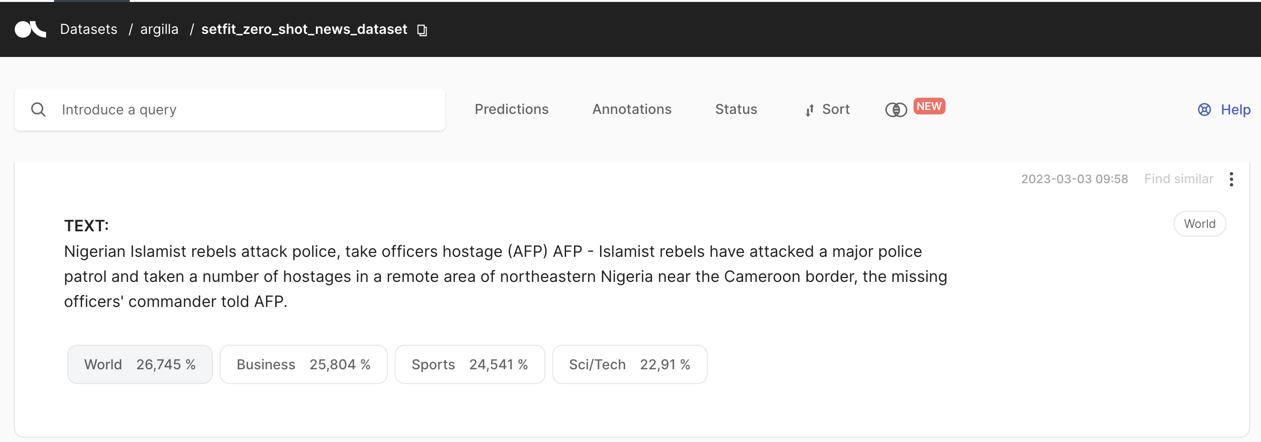
rg.log(name="setfit_zero_shot_news_dataset", records=setfit_zero_shot_news_dataset)
您可以在 Argilla UI 中访问 setfit_zero_shot_news_dataset
[15]:
f1_setfit_zero_shot = f1("setfit_zero_shot_news_dataset")
f1_setfit_zero_shot.visualize()
现在我们已经计算了每个模型的 F1 分数,我们可以创建一个比较表
[16]:
f_score = list(f1_setfit_zero_shot.data.keys())
f1_setfit_zero_shot_values = list(f1_setfit_zero_shot.data.values())
f1_zero_shot_values = list(f1_zero_shot.data.values())

unnecessary_labels = ["Sports_recall", "World_recall", ""]

df_results = pd.DataFrame({"f_score": f_score, "zero-shot classification": f1_zero_shot_values, "zero-shot SetFit classification": f1_setfit_zero_shot_values})
[17]:
df_results
[17]:
| f_score | 零样本分类 | 零样本 SetFit 分类 | |
|---|---|---|---|
| 0 | precision_macro | 0.517754 | 0.663322 |
| 1 | recall_macro | 0.529605 | 0.668816 |
| 2 | f1_macro | 0.514483 | 0.663725 |
| 3 | precision_micro | 0.529605 | 0.668816 |
| 4 | recall_micro | 0.529605 | 0.668816 |
| 5 | f1_micro | 0.529605 | 0.668816 |
| 6 | Sci/Tech_precision | 0.476950 | 0.556291 |
| 7 | Sci/Tech_recall | 0.283158 | 0.530526 |
| 8 | Sci/Tech_f1 | 0.355350 | 0.543103 |
| 9 | Sci/Tech_support | 11400.000000 | 7600.000000 |
| 10 | World_precision | 0.367909 | 0.663734 |
| 11 | World_recall | 0.358421 | 0.555789 |
| 12 | World_f1 | 0.363103 | 0.604984 |
| 13 | World_support | 11400.000000 | 7600.000000 |
| 14 | Business_precision | 0.449227 | 0.620098 |
| 15 | Business_recall | 0.565789 | 0.665789 |
| 16 | Business_f1 | 0.500815 | 0.642132 |
| 17 | Business_support | 11400.000000 | 7600.000000 |
| 18 | Sports_precision | 0.776930 | 0.813166 |
| 19 | Sports_recall | 0.911053 | 0.923158 |
| 20 | Sports_f1 | 0.838663 | 0.864678 |
| 21 | Sports_support | 11400.000000 | 7600.000000 |
结果解释: 毫无疑问,使用 SetFit 模型的零样本分类更有效。每个类别的 F1 分数都更好。
对于两个分类器,最佳预测类别都是 Sports。