📸 批量标注多模态数据#
在本教程中,我们将处理图像和文本的多模态数据。它将引导您完成以下步骤
加载包含电子产品图像和文本的数据集。
体验零样本图像和文本分类。
使用批量标注以及图像和文本嵌入来标注数据。
在标注的数据上训练 SetFit 分类模型。
运行 Argilla#
对于本教程,您需要运行 Argilla 服务器。部署和运行 Argilla 有两个主要选项
在 Hugging Face Spaces 上部署 Argilla:如果您在 Hugging Face 上有帐户,这是最快的选项,也是连接到外部 Notebook(例如,Google Colab)的推荐选择。
使用 Argilla 的快速入门 Docker 镜像启动 Argilla:如果您想在本地机器上运行 Argilla,这是推荐的选项。请注意,此选项仅允许您在本地运行教程,而不能与外部 Notebook 服务一起运行。
有关部署选项的更多信息,请查看文档的部署部分。
提示
本教程是一个 Jupyter Notebook。有两种运行方式
使用此页面顶部的“在 Colab 中打开”按钮。此选项允许您直接在 Google Colab 上运行 Notebook。不要忘记将运行时类型更改为 GPU,以加快模型训练和推理速度。
通过单击页面顶部的“查看源码”链接下载 .ipynb 文件。此选项允许您下载 Notebook 并在本地机器或您选择的 Jupyter Notebook 工具上运行它。
设置#
对于本教程,您需要使用 pip 安装 Argilla 客户端和一些第三方库
简介#
真实世界的多模态数据通常是文本和图像的混合。在本教程中,我们将使用电子产品的数据集。该数据集包含产品的图像和产品描述。
此 Notebook 使用来自虚构电子产品网店的电子零件和产品数据集。
让我们开始吧!
[2]:
%pip install argilla "setfit~=0.2.0" "datasets~=2.3.0" transformers sentence-transformers -qqq
让我们导入 Argilla 模块以进行数据读取和写入
[1]:
import argilla as rg
如果您使用 Docker 快速入门镜像或 Hugging Face Spaces 运行 Argilla,则需要使用 URL 和 API_KEY 初始化 Argilla 客户端
[ ]:
# Replace api_url with the url to your HF Spaces URL if using Spaces
# Replace api_key if you configured a custom API key
rg.init(
    api_url="https://:6900",
    api_key="admin.apikey"
)
如果您运行的是私有的 Hugging Face Space,您还需要按如下所示设置 HF_TOKEN
[ ]:
# # Set the HF_TOKEN environment variable
# import os
# os.environ['HF_TOKEN'] = "your-hf-token"

# # Replace api_url with the url to your HF Spaces URL
# # Replace api_key if you configured a custom API key
# rg.init(
#     api_url="https://[your-owner-name]-[your_space_name].hf.space",
#     api_key="admin.apikey",
#     extra_headers={"Authorization": f"Bearer {os.environ['HF_TOKEN']}"},
# )
最后,让我们包含我们需要的导入
[ ]:
import os
import pprint as pp
from requests import get

from datasets import load_dataset
from PIL import Image
from sklearn.metrics import accuracy_score
from sentence_transformers import SentenceTransformer
from transformers import pipeline
from sentence_transformers.losses import CosineSimilarityLoss
from setfit import SetFitModel, SetFitTrainer
from PIL import Image
启用遥测#
我们从您与教程的互动中获得宝贵的见解。为了改进我们为您提供最合适内容的方式,使用以下代码行将帮助我们了解本教程是否有效地为您服务。虽然这是完全匿名的,但如果您愿意,可以选择跳过此步骤。有关更多信息,请查看遥测页面。
[ ]:
try:
    from argilla.utils.telemetry import tutorial_running
    tutorial_running()
except ImportError:
    print("Telemetry is introduced in Argilla 1.20.0 and not found in the current installation. Skipping telemetry.")
“真实世界”的多模态数据集#
数据集样本包含 page_name、page_descriptions 和 label。数据集分为两个部分:labelled 和 unlabelled。“labelled” 部分是我标注的结果,因此我们可以测试方法。实际上,假设这不存在 😏。
[ ]:
ELECTRONICS_DATASET = "burtenshaw/electronics"
dataset = load_dataset(ELECTRONICS_DATASET)
labels = dataset["labelled"].features["label"].names
int2str = dataset["labelled"].features["label"].int2str
[12]:
# show a sample
pp.pprint(next(iter(dataset["labelled"])))
{'image_url': 'https://tse1.mm.bing.net/th?id=OIP.to3Cddhws6ECl-_ySZ5ShQHaFi&pid=Api',
 'label': 1,
 'page_description': '\n'
                     '\n'
                     'Are you looking for a way to reduce the number of '
                     'purchase orders you need to place for cable assemblies? '
                     "If so, then this guide is for you! We'll show you how to "
                     'source cable assemblies with fewer purchase orders, '
                     "saving you time and money. We'll cover topics such as "
                     'understanding the different types of cable assemblies, '
                     'researching suppliers, and negotiating the best prices. '
                     "We'll also provide tips on how to streamline the "
                     'ordering process and ensure you get the best quality '
                     "products. With this guide, you'll be able to source "
                     'cable assemblies with fewer purchase orders and get the '
                     'most out of your budget.',
 'page_name': 'How to Source Cable Assemblies With Fewer Purchase Orders ...'}
🔫 零样本分类#
📷 图像#
首先,我们将探索一些零样本技术。为了便于比较,我们将使用数据集的 labelled 部分。
[ ]:
# to save time, we'll take a slice of the dataset
test_dataset = load_dataset(ELECTRONICS_DATASET, split="test[:20%]")
[ ]:
# More models in the model hub.
model_name = "openai/clip-vit-large-patch14"
classifier = pipeline("zero-shot-image-classification", model = model_name)
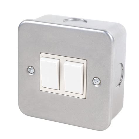
首先,我们可以对数据集中的一个图像进行零样本分类
[15]:
image_to_classify = next(iter(dataset["test"]))["image_url"]
scores = classifier(image_to_classify, candidate_labels = labels)
# show a sample
pp.pprint(scores[0])
Image.open(get(image_to_classify, stream =True).raw)
{'label': 'switches', 'score': 0.9631496667861938}
[15]:
现在,我们将测试零样本图像分类器在 labelled 部分数据集的子部分上的准确性和延迟。
[16]:
%%time
def classify_image(sample):
    label = classifier(sample["image_url"], candidate_labels = labels)[0]["label"]
    sample["clip_zero_shot"] = labels.index(label)
    return sample

test_dataset = test_dataset.map(classify_image)
CPU times: user 9min 20s, sys: 1.19 s, total: 9min 21s
Wall time: 2min 28s
[17]:
zero_shot_image_accuracy = accuracy_score(test_dataset["label"], test_dataset["clip_zero_shot"])
print(f"Accuracy: {zero_shot_image_accuracy}")
Accuracy: 0.8235294117647058
😞 使用 CLIP 模型的零样本图像分类在不到 2 分钟的时间内,仅对 20% 的测试数据给出了 0.82 的准确率。这个分数并不令人印象深刻。让我们看看文本是否更可靠。
📚 文本#
产品描述和名称也包含有价值的信息。让我们看看对这些信息进行零样本分类可以达到什么效果。
[18]:
classifier = pipeline(model="facebook/bart-large-mnli")
Downloading (…)lve/main/config.json: 100%|█████████████████████████████████████████████████████████████████████████████████████████████████████████████████████████████████████████████████████████████████████████████████████████████████████████████████████████████████████████████████████████████████████████████████████████████████████████████████████████████████████████████████████████████████████████████████████████████████████████████████████████████████████████████████████████████████████████████████████████████████████████████████████████████████████████████████████████████████████████████████████████████████████████████████████████████████████████████████████████████████████████████████████████████████████████████████████████████████████████████████████████████████████████████████████████████████████████████████████████████████████████████████████████████████████████████████████████████████████████████████████████████████████████████████████████| 1.15k/1.15k [00:00<00:00, 711kB/s]
Downloading pytorch_model.bin: 100%|███████████████████████████████████████████████████████████████████████████████████████████████████████████████████████████████████████████████████████████████████████████████████████████████████████████████████████████████████████████████████████████████████████████████████████████████████████████████████████████████████████████████████████████████████████████████████████████████████████████████████████████████████████████████████████████████████████████████████████████████████████████████████████████████████████████████████████████████████████████████████████████████████████████████████████████████████████████████████████████████████████████████████████████████████████████████████████████████████████████████████████████████████████████████████████████████████████████████████████████████████████████████████████████████████████████████████████████████████████████████████████████████████████████████████████████████| 1.63G/1.63G [00:06<00:00, 243MB/s]
Downloading (…)okenizer_config.json: 100%|██████████████████████████████████████████████████████████████████████████████████████████████████████████████████████████████████████████████████████████████████████████████████████████████████████████████████████████████████████████████████████████████████████████████████████████████████████████████████████████████████████████████████████████████████████████████████████████████████████████████████████████████████████████████████████████████████████████████████████████████████████████████████████████████████████████████████████████████████████████████████████████████████████████████████████████████████████████████████████████████████████████████████████████████████████████████████████████████████████████████████████████████████████████████████████████████████████████████████████████████████████████████████████████████████████████████████████████████████████████████████████████████████████████████████████████| 26.0/26.0 [00:00<00:00, 16.5kB/s]
Downloading (…)olve/main/vocab.json: 100%|███████████████████████████████████████████████████████████████████████████████████████████████████████████████████████████████████████████████████████████████████████████████████████████████████████████████████████████████████████████████████████████████████████████████████████████████████████████████████████████████████████████████████████████████████████████████████████████████████████████████████████████████████████████████████████████████████████████████████████████████████████████████████████████████████████████████████████████████████████████████████████████████████████████████████████████████████████████████████████████████████████████████████████████████████████████████████████████████████████████████████████████████████████████████████████████████████████████████████████████████████████████████████████████████████████████████████████████████████████████████████████████████████████████████████████████| 899k/899k [00:02<00:00, 401kB/s]
Downloading (…)olve/main/merges.txt: 100%|██████████████████████████████████████████████████████████████████████████████████████████████████████████████████████████████████████████████████████████████████████████████████████████████████████████████████████████████████████████████████████████████████████████████████████████████████████████████████████████████████████████████████████████████████████████████████████████████████████████████████████████████████████████████████████████████████████████████████████████████████████████████████████████████████████████████████████████████████████████████████████████████████████████████████████████████████████████████████████████████████████████████████████████████████████████████████████████████████████████████████████████████████████████████████████████████████████████████████████████████████████████████████████████████████████████████████████████████████████████████████████████████████████████████████████████| 456k/456k [00:00<00:00, 1.40MB/s]
Downloading (…)/main/tokenizer.json: 100%|████████████████████████████████████████████████████████████████████████████████████████████████████████████████████████████████████████████████████████████████████████████████████████████████████████████████████████████████████████████████████████████████████████████████████████████████████████████████████████████████████████████████████████████████████████████████████████████████████████████████████████████████████████████████████████████████████████████████████████████████████████████████████████████████████████████████████████████████████████████████████████████████████████████████████████████████████████████████████████████████████████████████████████████████████████████████████████████████████████████████████████████████████████████████████████████████████████████████████████████████████████████████████████████████████████████████████████████████████████████████████████████████████████████████████████| 1.36M/1.36M [00:00<00:00, 2.81MB/s]
[19]:
%%time
def classify_text(sample):
    label = classifier(sample["page_description"], candidate_labels = labels)["labels"][0]
    sample["bart_zero_shot"] = labels.index(label)
    return sample

test_dataset = test_dataset.map(classify_text)
Accuracy: 0.8235294117647058
CPU times: user 5min 41s, sys: 1.29 s, total: 5min 42s
Wall time: 1min 33s
[20]:
zero_shot_text_accuracy = accuracy_score(test_dataset["label"], test_dataset["clip_zero_shot"])
print(f"Accuracy: {zero_shot_text_accuracy}")
Accuracy: 0.8235294117647058
😞 文本分类花费的时间更少,但准确率也更低,为 .79。这表明某些信息存在于图像中,但文本中没有。如果我们能够整合这些信息,那就太好了。🤞
此外,这两种方法都使用了消耗大量计算资源的大型语言模型。
整合数据标注#
以上两种零样本分类方法的分数表明,使用零样本方法完成此任务是可能的,但具有挑战性。
借助(我们修改后的)Argilla,我们可以重新标注数据集,并结合来自图像和文本的信息。然后,我们可以在数据集上执行少样本学习。
剧透:通过结合图像和文本中的信息,这应该比零样本方法给我们带来更好的分数。此外,我们生成的语言模型应该比零样本模型具有更低的延迟。
使用嵌入进行批量标注#
📷 图像#
现在我们可以使用 clip 模型获取数据集中图像的图像嵌入。然后,我们可以重复将向量添加到数据集的过程,但现在使用 image_vectors 键。
[ ]:
# Load CLIP model for image embedding
image_encoder = SentenceTransformer('clip-ViT-B-32')
[ ]:
def encode_image(image_url):
    # utility function to encode image
    image = Image.open(get(image_url, stream =True).raw)
    vector = image_encoder.encode(image).tolist()
    return vector

# Encode text field using batched computation
dataset = dataset.map(lambda sample: {"image_vectors": encode_image(sample["image_url"])})
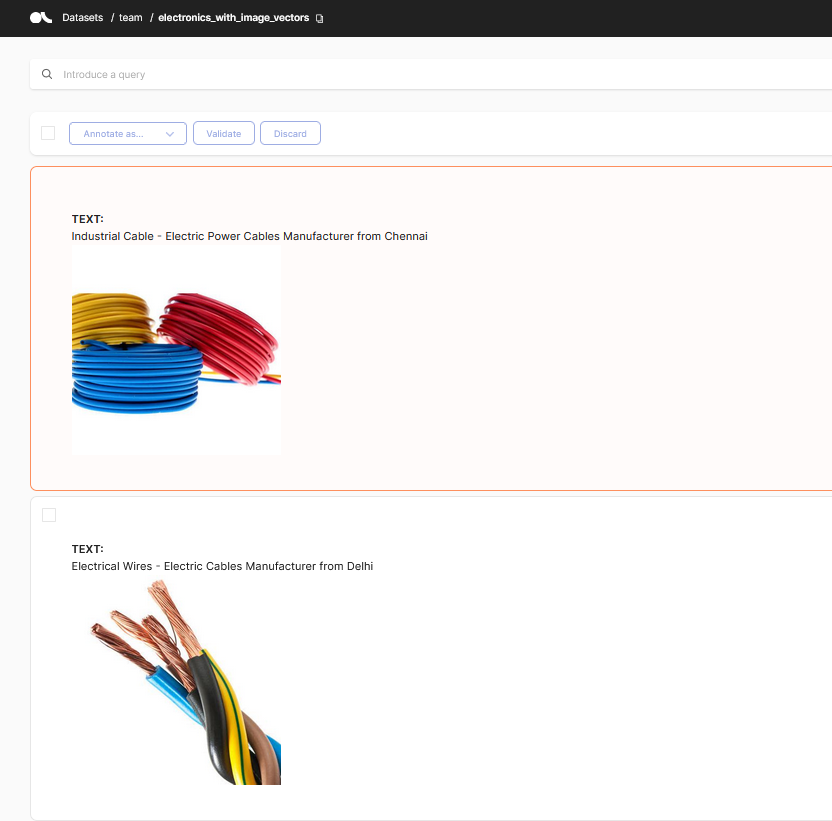
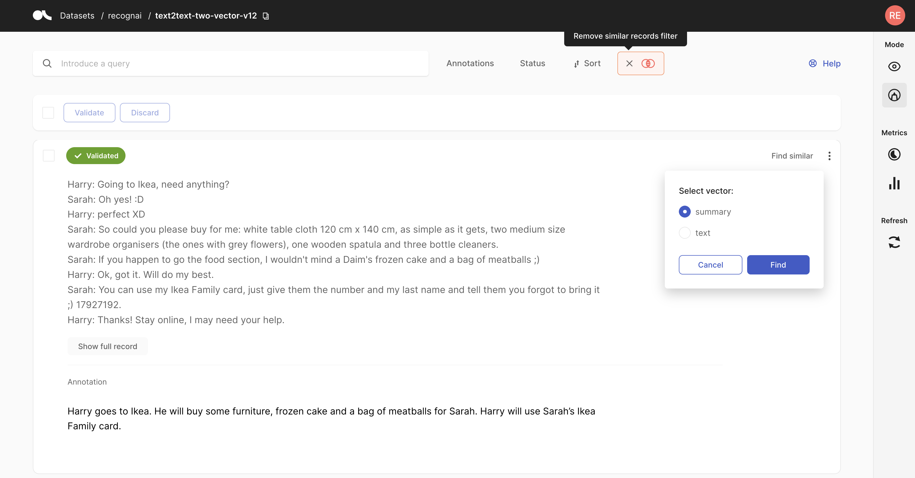
📚 文本#
借助 Argilla,我们可以使用语义搜索和“查找相似”按钮来标注样本。此处有关于此的完整教程:这里。它需要最近添加的相似性搜索功能。
[33]:
# Define sentence transformers model for text embedding
dataset = load_dataset(ELECTRONICS_DATASET, streaming=True, split="unlabelled")
encoder = SentenceTransformer("all-MiniLM-L6-v2")
[34]:
# Encode text field using batched computation
dataset = dataset.map(lambda batch: {"text_vectors": encoder.encode(batch["page_name"]).tolist()}, batch_size=32, batched=True)
上传到 Argilla#
我们可以将多个向量上传到 Argilla。我们只需要使用单独的键。我们将使用 image_vectors 和 text_vectors。
[37]:
# Turn vectors into a dictionary
dataset = dataset.map(
    lambda r: {"vectors": {"image": r["image_vectors"], "text": r["text_vectors"]}},
)
[ ]:
# we need to set the metadata field length to 200 for longer urls
os.environ["ARGILLA_METADATA_FIELD_LENGTH"] = "200"

# instantiate Argilla records with vectors
records = [
    rg.TextClassificationRecord(
        text=sample["page_name"],
        metadata=dict(_image_url=sample["image_url"]),
        vectors=sample["vectors"]
    )
    for sample in dataset
]
dataset_rg = rg.DatasetForTextClassification(records)

# upload recors with vectors to Argilla
rg.log(
    records=dataset_rg,
    name="electronics_with_vectors",
)

少样本分类#
我们现在可以使用新标注的数据集来训练分类器。由于样本数量有限,我们将使用 SetFit 模型。请注意,推理时间显着减少,准确率也提高了。
有关使用 SetFit 和 Argilla 进行少样本分类的完整教程,请参见这里。
[ ]:
# load the 'newly' labelled dataset
dataset_rg = rg.load("electronics_with_vectors")
labelled_dataset = dataset_rg.prepare_for_training(framework="transformers")
# # To try the prelabelled slice from HF Hub
# labelled_dataset = load_dataset(ELECTRONICS_DATASET, split="labelled")
# # To evaluate on the larger test set
# test_dataset = datasets.load_dataset(ELECTRONICS_DATASET, split="test")
[42]:
# Load SetFit model from Hub
model = SetFitModel.from_pretrained("sentence-transformers/paraphrase-mpnet-base-v2")

# Create trainer
trainer = SetFitTrainer(
    model=model,
    train_dataset=labelled_dataset,
    eval_dataset=test_dataset,
    loss_class=CosineSimilarityLoss,
    batch_size=16,
    num_iterations=10,
    column_mapping={"page_name":"text", "label":"label"}
)
model_head.pkl not found on HuggingFace Hub, initialising classification head with random weights. You should TRAIN this model on a downstream task to use it for predictions and inference.
现在让我们开始训练 ✈
[43]:
trainer.train()
metrics = trainer.evaluate()
Applying column mapping to training dataset
***** Running training *****
  Num examples = 5040
  Num epochs = 1
  Total optimization steps = 315
  Total train batch size = 16
Iteration: 100%|█████████████████████████████████████████████████████████████████████████████████████████████████████████████████████████████████████████████████████████████████████████████████████████████████████████████████████████████████████████████████████████████████████████████████████████████████████████████████████████████████████████████████████████████████████████████████████████████████████████████████████████████████████████████████████████████████████████████████████████████████████████████████████████████████████████████████████████████████████████████████████████████████████████████████████████████████████████████████████████████████████████████████████████████████████████████████████████████████████████████████████████████████████████████████████████████████████████████████████████████████████████████████████████████████████████████████████████████████████████████████████████████████████████████████████████████████████████████████████| 315/315 [00:53<00:00,  5.94it/s]
Epoch: 100%|█████████████████████████████████████████████████████████████████████████████████████████████████████████████████████████████████████████████████████████████████████████████████████████████████████████████████████████████████████████████████████████████████████████████████████████████████████████████████████████████████████████████████████████████████████████████████████████████████████████████████████████████████████████████████████████████████████████████████████████████████████████████████████████████████████████████████████████████████████████████████████████████████████████████████████████████████████████████████████████████████████████████████████████████████████████████████████████████████████████████████████████████████████████████████████████████████████████████████████████████████████████████████████████████████████████████████████████████████████████████████████████████████████████████████████████████████████████████████████████████| 1/1 [00:53<00:00, 53.04s/it]
Applying column mapping to evaluation dataset
***** Running evaluation *****
Downloading builder script: 100%|█████████████████████████████████████████████████████████████████████████████████████████████████████████████████████████████████████████████████████████████████████████████████████████████████████████████████████████████████████████████████████████████████████████████████████████████████████████████████████████████████████████████████████████████████████████████████████████████████████████████████████████████████████████████████████████████████████████████████████████████████████████████████████████████████████████████████████████████████████████████████████████████████████████████████████████████████████████████████████████████████████████████████████████████████████████████████████████████████████████████████████████████████████████████████████████████████████████████████████████████████████████████████████████████████████████████████████████████████████████████████████████████████████████████████████████████████| 4.20k/4.20k [00:00<00:00, 4.10MB/s]
{'accuracy': 0.9117647058823529}
[50]:
fewshot_relabelled_text_accuracy = metrics["accuracy"]
pp.pprint(fewshot_relabelled_text_accuracy)
0.9117647058823529
总结#
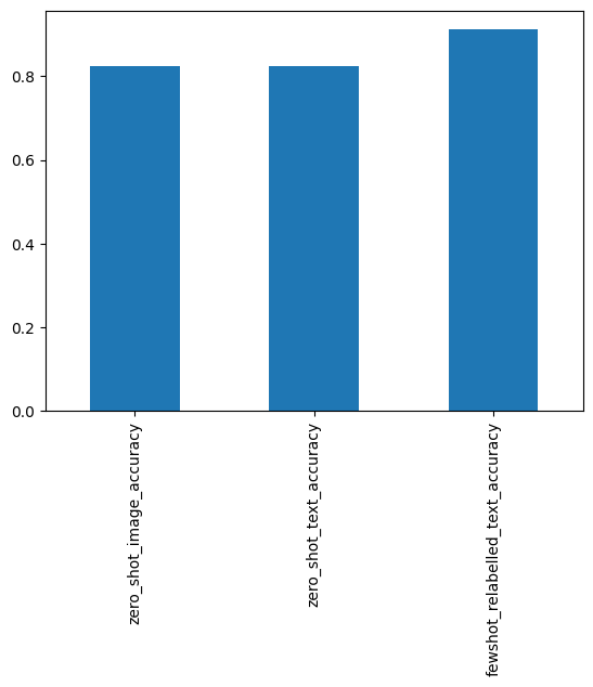
在本教程中,我们学习了如何使用 Argilla 的修改版本批量标注多模态数据集。我们将使用批量标注数据集训练的少样本分类器与图像和文本的零样本分类器进行了比较。结果表明,少样本分类器能够获得比零样本分类器更高的准确率。此外,SetFit 模型比零样本分类器快得多。
这种方法可以应用于数据有限的分类任务,并且可以用于以最少的人工工作量训练分类器。
[54]:
from pandas import Series

Series(
    dict(
        zero_shot_image_accuracy=zero_shot_image_accuracy,
        zero_shot_text_accuracy=zero_shot_text_accuracy,
        fewshot_relabelled_text_accuracy=fewshot_relabelled_text_accuracy,
    )
).plot.bar()
[54]:
<Axes: >