🧱 使用 Sentence Transformers 增强弱监督规则#
在本教程中,我们将展示如何在 Argilla 中使用句子嵌入扩展弱监督工作流。我们从 Argilla 弱监督教程 中介绍的弱监督工作流开始,并通过扩展其规则的覆盖范围来改进其结果。
✍️ 我们定义规则并为 ag_news 数据集生成弱标签。
🧱 我们使用来自 Sentence Transformers 库的句子嵌入来扩展我们的弱标签。
📰 最后,我们使用标签模型生成数据,用于训练下游模型作为新闻分类器。
🚀 通过简单地扩展我们的弱标签,我们在准确率上实现了 4% 的提升。
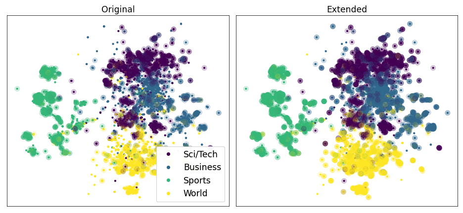
上面的两个图表显示了在使用嵌入扩展弱标签之前和之后的覆盖率。每个点对应于 ag news 测试集中的一个示例。颜色表示示例的相应类别。透明圆圈中的点至少被一个规则覆盖。
简介#
标注函数通常具有高精度,但覆盖率较低。只有严格匹配给定函数所确定条件的记录才会被标注,而其他潜在的候选记录将被排除在外。
基于 Hazy Research 小组的发现,我们提出了一种通过使用句子嵌入扩展标注函数产生的弱标签来解决此问题的方法。
我们通过给未标注的记录赋予与其在嵌入空间中最接近的已标注邻居相同的标签来扩展标注函数的覆盖率,前提是它们之间的余弦相似度得分高于某个阈值。
在本教程中,我们将展示,通过调整这些相似度阈值并选择合适的句子嵌入,我们能够显着提高弱监督工作流产生的下游分类器的准确率。
运行 Argilla#
对于本教程,您需要运行 Argilla 服务器。部署和运行 Argilla 有两个主要选项
在 Hugging Face Spaces 上部署 Argilla:如果您想使用外部 notebook(例如,Google Colab)运行教程,并且您在 Hugging Face 上有一个帐户,您只需点击几下即可在 Spaces 上部署 Argilla

有关配置部署的详细信息,请查看 Hugging Face Hub 官方指南。
使用 Argilla 的快速入门 Docker 镜像启动 Argilla:如果您想在 本地机器上运行 Argilla,这是推荐选项。请注意,此选项仅允许您在本地运行本教程,而不能使用外部 notebook 服务。
有关部署选项的更多信息,请查看文档的部署部分。
提示
本教程是一个 Jupyter Notebook。有两种选项可以运行它
使用此页面顶部的“在 Colab 中打开”按钮。此选项允许您直接在 Google Colab 上运行 notebook。不要忘记将运行时类型更改为 GPU 以加快模型训练和推理速度。
通过单击页面顶部的“查看源代码”链接下载 .ipynb 文件。此选项允许您下载 notebook 并在本地机器或您选择的 Jupyter notebook 工具上运行它。
设置#
对于本教程,您需要使用 pip 安装 Argilla 客户端和一些第三方库
[ ]:
%pip install argilla faiss-cpu sentence_transformers transformers datasets snorkel -qqq
让我们导入 Argilla 模块以进行数据读取和写入
[4]:
import argilla as rg
如果您使用 Docker 快速入门镜像或公共 Hugging Face Spaces 运行 Argilla,则需要使用 URL 和 API_KEY 初始化 Argilla 客户端
[5]:
# Replace api_url with the url to your HF Spaces URL if using Spaces
# Replace api_key if you configured a custom API key
rg.init(
    api_url="https://:6900",
    api_key="admin.apikey"
)
如果您运行的是私有 Hugging Face Space,您还需要按如下方式设置 HF_TOKEN
[ ]:
# # Set the HF_TOKEN environment variable
# import os
# os.environ['HF_TOKEN'] = "your-hf-token"

# # Replace api_url with the url to your HF Spaces URL
# # Replace api_key if you configured a custom API key
# rg.init(
#     api_url="https://[your-owner-name]-[your_space_name].hf.space",
#     api_key="admin.apikey",
#     extra_headers={"Authorization": f"Bearer {os.environ['HF_TOKEN']}"},
# )
现在让我们添加所需的导入
[16]:
from datasets import load_dataset
from argilla.labeling.text_classification import Rule, add_rules, WeakLabels, Snorkel
from sentence_transformers import SentenceTransformer
from tqdm.auto import tqdm
启用遥测#
我们从您与我们的教程的互动中获得宝贵的见解。为了改进我们自己,为您提供最合适的内容,使用以下代码行将帮助我们了解本教程是否有效地为您服务。虽然这是完全匿名的,但如果您愿意,可以选择跳过此步骤。有关更多信息,请查看 遥测 页面。
[ ]:
try:
    from argilla.utils.telemetry import tutorial_running
    tutorial_running()
except ImportError:
    print("Telemetry is introduced in Argilla 1.20.0 and not found in the current installation. Skipping telemetry.")
详细工作流#
使用句子嵌入执行弱监督的典型工作流程是
使用您的原始数据集创建 Argilla 数据集。如果您有一些已标注的数据,您可以将其记录到同一数据集中。
使用 UI 中的“规则定义”模式定义一组弱标注规则。
创建一个
WeakLabels对象并应用规则。您可以从数据集中加载规则,并使用 Python 添加其他规则和标注函数。通常,您会在步骤 2 和此步骤之间迭代。通过为每个记录(矩阵的行)提供句子嵌入和为每个规则(矩阵的列)提供相似度阈值来扩展
WeakLabels对象。对扩展的弱标签感到满意后,将
WeakLabels实例的扩展矩阵与您选择的库/方法一起使用,以构建训练集,甚至训练下游文本分类模型。您可以在此步骤和步骤 4 之间迭代,尝试多个阈值和嵌入可能性,直到获得令人满意的结果。
本指南向您展示了一个使用 Snorkel 的端到端示例。您也可以选择使用 Argilla 中提供的任何其他标签模型。如果您有兴趣了解其他选项,请查看我们的 弱监督指南。
数据集#
我们将使用 ag_news 数据集,这是一个著名的基准文本分类模型。
但是,为了保证公平的比较,我们将在验证集上优化阈值,并将测试集留作最终评估。
[17]:
agnews = load_dataset("ag_news")

agnews_train, agnews_valid = (
    agnews["train"].train_test_split(test_size=4000, seed=43).values()
)
WARNING:datasets.builder:Found cached dataset ag_news (/root/.cache/huggingface/datasets/ag_news/default/0.0.0/bc2bcb40336ace1a0374767fc29bb0296cdaf8a6da7298436239c54d79180548)
1. 创建包含未标注数据和测试数据的 Argilla 数据集#
让我们将已标注和未标注的记录集加载到 Argilla 中。
[18]:
# build our labelled records to evaluate our heuristic rules and optimize the thresholds
records = [
    rg.TextClassificationRecord(
        text=record["text"],
        metadata={"split": "labelled"},
        annotation=agnews_valid.features["label"].int2str(record["label"]),
        id=f"valid_{idx}",
    )
    for idx, record in enumerate(agnews_valid)
]

# build our unlabelled records
records += [
    rg.TextClassificationRecord(
        text=record["text"],
        metadata={"split": "unlabelled"},
        id=f"train_{idx}",
    )
    for idx, record in enumerate(agnews_train.select(range(8000)))
]

# log the records to Argilla
rg.log(records, name="agnews")
12000 records logged to https://dvilasuero-argilla-space-52456aa.hf.space/datasets/team/agnews
[18]:
BulkResponse(dataset='agnews', processed=12000, failed=0)
完成此步骤后,您将拥有一个完全可浏览的数据集,可以通过 Argilla Web 应用程序 访问它。
2. 定义规则#
我们将使用以下规则。
[19]:
# define queries and patterns for each category (using ES DSL)
queries = [
    (["money", "financ*", "dollar*"], "Business"),
    (["war", "gov*", "minister*", "conflict"], "World"),
    (["footbal*", "sport*", "game", "play*"], "Sports"),
    (["sci*", "techno*", "computer*", "software", "web"], "Sci/Tech"),
]

# define rules
rules = [Rule(query=term, label=label) for terms, label in queries for term in terms]
现在我们可以按如下方式将它们添加到数据集中
[20]:
add_rules(dataset="agnews", rules=rules)
3. 构建和分析弱标签#
从我们的规则构建弱标签后,它们的摘要显示如下
[21]:
# apply the rules to the dataset to obtain the weak labels
weak_labels = WeakLabels(dataset="agnews")
weak_labels.summary()
[21]:
| label | coverage | annotated_coverage | overlaps | conflicts | correct | incorrect | precision | |
|---|---|---|---|---|---|---|---|---|
| money | {Business} | 0.008000 | 0.00925 | 0.002750 | 0.002083 | 13 | 24 | 0.351351 |
| financ* | {Business} | 0.020667 | 0.02100 | 0.005417 | 0.004667 | 56 | 28 | 0.666667 |
| dollar* | {Business} | 0.016250 | 0.01550 | 0.003833 | 0.002750 | 42 | 20 | 0.677419 |
| war | {World} | 0.013750 | 0.01175 | 0.003000 | 0.001333 | 34 | 13 | 0.723404 |
| gov* | {World} | 0.045167 | 0.04000 | 0.011083 | 0.006000 | 76 | 84 | 0.475000 |
| minister* | {World} | 0.028917 | 0.03175 | 0.007167 | 0.002583 | 114 | 13 | 0.897638 |
| conflict | {World} | 0.003167 | 0.00300 | 0.001333 | 0.000250 | 10 | 2 | 0.833333 |
| footbal* | {Sports} | 0.014333 | 0.01475 | 0.005583 | 0.000333 | 53 | 6 | 0.898305 |
| sport* | {Sports} | 0.020750 | 0.02375 | 0.006250 | 0.001333 | 87 | 8 | 0.915789 |
| game | {Sports} | 0.039917 | 0.04150 | 0.013417 | 0.001917 | 132 | 34 | 0.795181 |
| play* | {Sports} | 0.055000 | 0.05875 | 0.016667 | 0.004500 | 168 | 67 | 0.714894 |
| sci* | {Sci/Tech} | 0.015833 | 0.01700 | 0.002583 | 0.001250 | 55 | 13 | 0.808824 |
| techno* | {Sci/Tech} | 0.028250 | 0.02900 | 0.008500 | 0.002667 | 82 | 34 | 0.706897 |
| computer* | {Sci/Tech} | 0.027917 | 0.02925 | 0.011583 | 0.004167 | 97 | 20 | 0.829060 |
| software | {Sci/Tech} | 0.031000 | 0.03225 | 0.009667 | 0.002500 | 104 | 25 | 0.806202 |
| web | {Sci/Tech} | 0.018250 | 0.01975 | 0.004417 | 0.001500 | 70 | 9 | 0.886076 |
| total | {Business, World, Sports, Sci/Tech} | 0.327583 | 0.33450 | 0.053667 | 0.017917 | 1193 | 400 | 0.748901 |
在接下来的步骤中,我们将尝试通过句子嵌入扩展我们的弱标签矩阵。通过这种方式,我们将增加规则的覆盖率,同时保持可接受的精度。
4. 使用弱标签#
使用 Snorkel 的标签模型#
Snorkel 的标签模型是迄今为止使用弱监督的最流行选项,Argilla 为其提供了内置支持。在这里,我们将我们的弱标签拟合到 Snorkel 标签模型,然后我们检查规则覆盖的记录的性能。
[22]:
# create the Snorkel label model
label_model = Snorkel(weak_labels)

# fit the model, for the learning rate and epochs we ran a quick grid search
label_model.fit(lr=0.002, n_epochs=10, progress_bar=False)

# evaluate the label model
print(label_model.score(output_str=True))
              precision    recall  f1-score   support

      Sports       0.79      0.95      0.86       380
    Sci/Tech       0.80      0.76      0.78       454
       World       0.70      0.82      0.75       257
    Business       0.69      0.40      0.50       247

    accuracy                           0.76      1338
   macro avg       0.74      0.73      0.72      1338
weighted avg       0.76      0.76      0.75      1338
5. 扩展弱标签#
让我们扩展我们的弱标签,看看这如何影响 Snorkel 标签模型的评估。
生成句子嵌入#
让我们为弱标签矩阵的每个记录生成句子嵌入。通过强大的通用预训练嵌入,或通过专门为手头任务的领域预训练的嵌入,将获得最佳结果。
在这里,我们选择来自著名的 Sentence Transformers 库 的 all-MiniLM-L6-v2 嵌入。Argilla 允许我们尝试来自任何来源的嵌入,只要它们以二维数组的形式提供给弱标签矩阵。
例如,除了 Sentence Transformers 之外,我们还可以使用 OpenAI 嵌入,或者来自 Tensorflow Hub 的文本嵌入。
[23]:
# instantiate the model for the sentence embeddings
# we strongly recommend using a GPU for the computation of the embeddings
model = SentenceTransformer("all-MiniLM-L6-v2", device="cpu")

# compute the embeddings and store them in a list
embeddings = []
for rec in tqdm(weak_labels.records()):
    embeddings.append(model.encode(rec.text))
设置阈值#
我们首先对哪些阈值适用于此特定弱标签矩阵做出有根据的猜测。我们将所有规则的阈值设置为 0.60。这意味着,对于每个规则,如果记录的余弦相似度高于此值,则该记录的标签将扩展到其最近的未标注邻居。
[24]:
thresholds = [0.6] * len(rules)
扩展弱标签矩阵#
我们通过提供阈值和句子嵌入来调用 extend_matrix 方法。
[25]:
weak_labels.extend_matrix(thresholds, embeddings)
随着弱标签矩阵的扩展,我们可以看到覆盖率上升了。
[26]:
weak_labels.summary()
[26]:
| label | coverage | annotated_coverage | overlaps | conflicts | correct | incorrect | precision | |
|---|---|---|---|---|---|---|---|---|
| money | {Business} | 0.017667 | 0.02025 | 0.009750 | 0.008083 | 43 | 38 | 0.530864 |
| financ* | {Business} | 0.037500 | 0.03800 | 0.016417 | 0.013917 | 99 | 53 | 0.651316 |
| dollar* | {Business} | 0.039667 | 0.04050 | 0.020583 | 0.017750 | 118 | 44 | 0.728395 |
| war | {World} | 0.031833 | 0.03125 | 0.015083 | 0.008250 | 81 | 44 | 0.648000 |
| gov* | {World} | 0.096083 | 0.08750 | 0.042000 | 0.024417 | 188 | 162 | 0.537143 |
| minister* | {World} | 0.053750 | 0.05350 | 0.023000 | 0.008083 | 197 | 17 | 0.920561 |
| conflict | {World} | 0.010583 | 0.00925 | 0.007833 | 0.003917 | 24 | 13 | 0.648649 |
| footbal* | {Sports} | 0.018333 | 0.01925 | 0.007833 | 0.000333 | 71 | 6 | 0.922078 |
| sport* | {Sports} | 0.036667 | 0.03900 | 0.014417 | 0.004000 | 142 | 14 | 0.910256 |
| game | {Sports} | 0.062417 | 0.06525 | 0.026750 | 0.004917 | 211 | 50 | 0.808429 |
| play* | {Sports} | 0.082417 | 0.08650 | 0.033833 | 0.011583 | 248 | 98 | 0.716763 |
| sci* | {Sci/Tech} | 0.023667 | 0.02500 | 0.003750 | 0.001917 | 80 | 20 | 0.800000 |
| techno* | {Sci/Tech} | 0.059667 | 0.05850 | 0.029833 | 0.019167 | 130 | 104 | 0.555556 |
| computer* | {Sci/Tech} | 0.052000 | 0.05250 | 0.029583 | 0.013750 | 165 | 45 | 0.785714 |
| software | {Sci/Tech} | 0.051917 | 0.05125 | 0.025667 | 0.010417 | 162 | 43 | 0.790244 |
| web | {Sci/Tech} | 0.036417 | 0.03650 | 0.015667 | 0.007167 | 121 | 25 | 0.828767 |
| total | {Business, World, Sports, Sci/Tech} | 0.523500 | 0.52525 | 0.134917 | 0.057917 | 2080 | 776 | 0.728291 |
我们还看到,我们规则的平均精度下降了(从 0.75 降至 0.66)。然而,这种下降可以通过我们的标签模型部分补偿。如果我们再次将弱标签拟合到 Snorkel 标签模型,我们可以看到,支持度显着提高,正如预期的那样,而准确率的下降幅度很小。
[27]:
label_model = Snorkel(weak_labels)
label_model.fit(lr=0.002, n_epochs=10, progress_bar=False)
print(label_model.score(output_str=True))
              precision    recall  f1-score   support

      Sports       0.81      0.95      0.87       550
    Sci/Tech       0.77      0.78      0.77       655
       World       0.70      0.84      0.76       468
    Business       0.72      0.38      0.50       428

    accuracy                           0.76      2101
   macro avg       0.75      0.74      0.73      2101
weighted avg       0.75      0.76      0.74      2101
您可以查看 附录,以详细了解弱标签矩阵如何在后台扩展。
我们建议以某种方式优化阈值以获得最高的性能提升,而不是使用通用的固定阈值。我们在 附录 中详细描述的优化产生了以下阈值
[28]:
optimized_thresholds = [
    0.4,
    0.4,
    0.6,
    0.4,
    0.5,
    0.8,
    1.0,
    0.4,
    0.4,
    0.5,
    0.6,
    0.4,
    0.4,
    0.6,
    0.6,
    0.8,
]
每次使用阈值和嵌入调用 extend_matrix 都会构建一个 faiss 索引,该索引将被缓存在弱标签对象中。
如果我们在下次调用 extend_matrix 时不提供嵌入,则将重新利用此索引,并且新的扩展矩阵将替换当前的扩展矩阵。因此,使用新阈值扩展矩阵非常便宜。
[29]:
weak_labels.extend_matrix(optimized_thresholds)
label_model = Snorkel(weak_labels)
label_model.fit(lr=0.002, n_epochs=10, progress_bar=False)
print(label_model.score(output_str=True))
              precision    recall  f1-score   support

      Sports       0.87      0.90      0.88       883
    Sci/Tech       0.69      0.72      0.70       880
       World       0.78      0.74      0.76       751
    Business       0.64      0.62      0.63       826

    accuracy                           0.75      3340
   macro avg       0.74      0.74      0.74      3340
weighted avg       0.75      0.75      0.75      3340
优化的阈值似乎进一步降低了标签模型的准确率,但也显着提高了覆盖率。
6. 训练下游模型#
现在,我们将训练与 之前的教程 中相同的下游模型,但基于由我们扩展的弱标签的标签模型生成的数据。
首先,让我们定义一个辅助函数,它基本上是先前教程中的复制粘贴。
[30]:
import pandas as pd
from sklearn.feature_extraction.text import CountVectorizer
from sklearn.naive_bayes import MultinomialNB
from sklearn.pipeline import Pipeline
from sklearn import metrics


def train_and_evaluate_downstream_model(label_model):
    """
    Train a downstream model with the predictions of a label model and
    evaluate it with the test split of the ag news dataset
    """
    # get records with the predictions from the label model
    records = label_model.predict()

    # turn str labels into integers
    label2int = label_model.weak_labels.label2int

    # extract training data
    X_train = [rec.text for rec in records]
    y_train = [label2int[rec.prediction[0][0]] for rec in records]

    # define our final classifier
    classifier = Pipeline([("vect", CountVectorizer()), ("clf", MultinomialNB())])

    # fit the classifier
    classifier.fit(
        X=X_train,
        y=y_train,
    )

    # extract text and labels
    X_test = [rec["text"] for rec in agnews["test"]]
    y_test = [
        label2int[agnews["test"].features["label"].int2str(rec["label"])]
        for rec in agnews["test"]
    ]

    # get predictions for the test set
    predicted = classifier.predict(X_test)

    return metrics.classification_report(
        y_test, predicted, target_names=[k for k in label2int.keys() if k]
    )
现在让我们看看我们的下游模型与 之前的教程 中的原始模型相比如何。请记住,我们实现了约 82% 的准确率。
[31]:
print(train_and_evaluate_downstream_model(label_model))
              precision    recall  f1-score   support

      Sports       0.88      0.96      0.92      1900
    Sci/Tech       0.77      0.82      0.79      1900
       World       0.86      0.84      0.85      1900
    Business       0.82      0.71      0.76      1900

    accuracy                           0.83      7600
   macro avg       0.83      0.83      0.83      7600
weighted avg       0.83      0.83      0.83      7600
现在,使用我们扩展的弱标签矩阵,我们能够实现 86% 的准确率,比我们最初的方法提高了 4%。
总结#
在本教程中,您已经了解了如何使用词嵌入改进 Argilla 中的弱监督工作流。通过对原始工作流进行非常小的更改,我们能够显着提高下游模型的准确率。这表明 Argilla 可以大大减少人工标注者在编写规则之前需要付出的努力,然后才能取得卓越的成果。
附录:可视化更改#
让我们可视化弱标签矩阵如何在单行中扩展。
[32]:
import pandas as pd


def get_transitions(weak_labels, idx):
    transitions = list(
        list(zip(row[0], row[1]))
        for row in zip(weak_labels._matrix, weak_labels._extended_matrix)
    )
    transitions = transitions[idx]
    label_dict = weak_labels.int2label
    rule_labels = weak_labels.summary().reset_index()["index"].values.tolist()[:-1]
    transitions_df = []
    for rule_idx, rule in enumerate(rule_labels):
        old_label = transitions[rule_idx][0]
        new_label = transitions[rule_idx][1]
        transitions_df.append(
            {
                "rule": rule,
                "old label": label_dict[old_label],
                "new label": label_dict[new_label],
            }
        )
    transitions_df = pd.DataFrame(transitions_df)
    text = weak_labels.records()[idx].text
    return transitions_df, text


transitions, text = get_transitions(weak_labels, 15)
通过阅读选定的记录,我们可以清楚地注意到这是一篇关于世界政治的新闻文章,因此应归类为 World。
[33]:
text
[33]:
'Nicaragua tells US it will destroy its antiaircraft missiles MANAGUA, Nicaragua -- President Enrique Bolanos told US Defense Secretary Donald H. Rumsfeld yesterday that Nicaragua would completely eliminate a stockpile of hundreds of surface-to-air missiles with no expectation of compensation from the United States.'
让我们将此记录的原始弱标签矩阵的行("old label" 行)和扩展后的同一行("new label" 行)并排放置。
我们看到,这篇新闻文章在原始矩阵中未被我们的任何规则标注。
但是,它是两个 Business 文章的最近未标注邻居,与规则 financ* 和 dollar* 匹配,并且其与它们的相似度得分高于我们选择的阈值。对于两个 World 文章,与规则 war 和 minister* 匹配,以及对于一个与规则 sci* 匹配的 Sci/Tech 文章,也发生了同样的情况。
[34]:
transitions.transpose()
[34]:
| 0 | 1 | 2 | 3 | 4 | 5 | 6 | 7 | 8 | 9 | 10 | 11 | 12 | 13 | 14 | 15 | |
|---|---|---|---|---|---|---|---|---|---|---|---|---|---|---|---|---|
| rule | money | financ* | dollar* | war | gov* | minister* | conflict | footbal* | sport* | game | play* | sci* | techno* | computer* | software | web |
| old label | None | None | None | None | None | None | None | None | None | None | None | None | None | None | None | None |
| new label | None | None | None | None | None | None | None | None | None | None | None | None | None | None | None | None |
附录:优化阈值#
每次使用阈值和嵌入调用 extend_matrix 都会构建一个 faiss 索引,该索引将被缓存在弱标签对象中。
如果我们在下次调用 extend_matrix 时不提供嵌入,则将重新利用此索引,并且新的扩展矩阵将替换当前的扩展矩阵。这个新矩阵是根据我们的新相似度阈值对原始弱标签矩阵进行的扩展。
[35]:
# Let's try to set all thresholds to 0.8 instead of 0.6.
thresholds = [0.8] * len(rules)

# As we have already generated the index in our first call, we just need to provide the thresholds.
weak_labels.extend_matrix(thresholds)
有几种不同的方法可以找到扩展弱标签矩阵的最佳相似度阈值:我们将从计算成本最低到最高的顺序进行列出。
1. 阻止低重叠规则的扩展#
在将所有相似度阈值设置为合理值后,优化单个级别的相似度阈值的一个好方法是阻止低重叠规则的扩展,因为它们在扩展后更可能产生不准确的结果。
[36]:
summary = weak_labels.summary(normalize_by_coverage=True).reset_index().head(len(rules))
summary = summary.rename(columns={"index": "rule"})
summary = summary.sort_values(by="overlaps", ascending=True)[["rule", "overlaps"]]
summary = summary.reset_index()
summary
[36]:
| index | rule | overlaps | |
|---|---|---|---|
| 0 | 11 | sci* | 0.158974 |
| 1 | 3 | war | 0.208092 |
| 2 | 2 | dollar* | 0.235577 |
| 3 | 4 | gov* | 0.236427 |
| 4 | 15 | web | 0.240664 |
| 5 | 5 | minister* | 0.244382 |
| 6 | 1 | financ* | 0.257692 |
| 7 | 8 | sport* | 0.287823 |
| 8 | 12 | techno* | 0.295580 |
| 9 | 10 | play* | 0.299259 |
| 10 | 14 | software | 0.303030 |
| 11 | 9 | game | 0.334694 |
| 12 | 0 | money | 0.340000 |
| 13 | 7 | footbal* | 0.380682 |
| 14 | 13 | computer* | 0.401662 |
| 15 | 6 | conflict | 0.404762 |
[37]:
thresholds = [0.6] * len(rules)

# Let's block the extension of the top 5 rules with the least overlap.
turn_off_index = summary["index"][0:6]

# We block the extension of a rule by setting its similarity threshold to 1.0.
for rule_index in turn_off_index:
    thresholds[rule_index] = 1.0

weak_labels.extend_matrix(thresholds)
label_model = Snorkel(weak_labels)
label_model.fit(lr=0.002, n_epochs=10, progress_bar=False)
print(train_and_evaluate_downstream_model(label_model))
              precision    recall  f1-score   support

      Sports       0.79      0.99      0.88      1900
    Sci/Tech       0.60      0.83      0.70      1900
       World       0.81      0.84      0.82      1900
    Business       0.91      0.31      0.46      1900

    accuracy                           0.74      7600
   macro avg       0.78      0.74      0.72      7600
weighted avg       0.78      0.74      0.72      7600
2. 暴力破解:在标签模型上进行网格搜索#
在这种方法中,我们将所有阈值设置为初始值,然后网格搜索每个阈值的最佳值。然后,我们优化开发集中标签模型的覆盖率和准确率之间的调和平均值。这将确保我们选择在两个指标之间具有最佳权衡的阈值。
我们获得了与先前方法相同的改进,在测试集上的最终准确率为 86%。
[38]:
def train_eval_labelmodel(ths):
    weak_labels.extend_matrix(ths)

    label_model = Snorkel(weak_labels)
    label_model.fit(lr=0.002, n_epochs=10, progress_bar=False)

    metrics = label_model.score()
    acc, sup, n = (
        metrics["accuracy"],
        metrics["macro avg"]["support"],
        len(weak_labels.annotation()),
    )
    coverage = sup / n
    return 2 * acc * coverage / (acc + coverage)
[39]:
import copy
from tqdm.auto import tqdm
import numpy as np

ths_range = np.arange(1, 0.3, -0.1)
n_ths = len(weak_labels.rules)

best_thresholds = [1.0] * n_ths
best_acc = 0.0
for i in tqdm(range(n_ths), total=n_ths):
    thresholds = best_thresholds.copy()
    for threshold in ths_range:
        thresholds[i] = threshold
        acc = train_eval_labelmodel(thresholds)
        if acc > best_acc:
            best_acc = acc
            best_thresholds = thresholds.copy()
[40]:
np.array(best_thresholds)
[40]:
array([0.4, 0.4, 0.4, 0.4, 0.4, 0.5, 1. , 0.4, 0.4, 0.4, 0.5, 0.4, 0.4,
       0.4, 0.5, 0.4])
[41]:
weak_labels.extend_matrix(best_thresholds)
label_model = Snorkel(weak_labels)
label_model.fit(lr=0.002, n_epochs=10, progress_bar=False)
print(train_and_evaluate_downstream_model(label_model))
              precision    recall  f1-score   support

      Sports       0.89      0.97      0.93      1900
    Sci/Tech       0.62      0.88      0.73      1900
       World       0.79      0.88      0.83      1900
    Business       0.90      0.33      0.48      1900

    accuracy                           0.77      7600
   macro avg       0.80      0.77      0.74      7600
weighted avg       0.80      0.77      0.74      7600
3. 暴力破解:在下游模型上进行网格搜索#
在这里,我们再次将所有阈值设置为初始值,并网格搜索每个单独阈值的最佳值,但现在我们优化开发集中下游模型的准确率。我们在测试集上获得了 85% 的最终准确率,略低于我们通过先前方法获得的准确率。
[42]:
# retrieve records with annotations
test_ds = weak_labels.records(has_annotation=True)

# extract text and labels
X_test_for_grid_search = [rec.text for rec in test_ds]
y_test_for_grid_search = [weak_labels.label2int[rec.annotation] for rec in test_ds]


def train_eval_downstream(ths):
    weak_labels.extend_matrix(ths)

    label_model = Snorkel(weak_labels)
    label_model.fit(lr=0.002, n_epochs=10, progress_bar=False)

    records = label_model.predict()

    X_train = [rec.text for rec in records]
    y_train = [weak_labels.label2int[rec.prediction[0][0]] for rec in records]

    classifier = Pipeline([("vect", CountVectorizer()), ("clf", MultinomialNB())])

    classifier.fit(
        X=X_train,
        y=y_train,
    )

    accuracy = classifier.score(
        X=X_test_for_grid_search,
        y=y_test_for_grid_search,
    )

    return accuracy
[43]:
from copy import copy
from tqdm.auto import tqdm

best_thresholds, best_acc = [1.0] * len(weak_labels.rules), 0
ths_range = np.arange(1, 0.3, -0.1)
n_ths = len(weak_labels.rules)

for i in tqdm(range(n_ths), total=n_ths):
    thresholds = best_thresholds.copy()
    for threshold in ths_range:
        thresholds[i] = threshold
        acc = train_eval_downstream(thresholds)
        if acc > best_acc:
            best_acc = acc
            best_thresholds = thresholds.copy()
[44]:
np.array(best_thresholds)
[44]:
array([0.4, 0.6, 0.6, 0.5, 1. , 0.6, 0.6, 0.5, 0.5, 0.5, 1. , 0.4, 1. ,
       0.7, 1. , 0.9])
[45]:
weak_labels.extend_matrix(best_thresholds)
label_model = Snorkel(weak_labels)
label_model.fit(lr=0.002, n_epochs=10, progress_bar=False)
print(train_and_evaluate_downstream_model(label_model))
              precision    recall  f1-score   support

      Sports       0.86      0.97      0.91      1900
    Sci/Tech       0.79      0.77      0.78      1900
       World       0.88      0.82      0.85      1900
    Business       0.77      0.75      0.76      1900

    accuracy                           0.83      7600
   macro avg       0.82      0.83      0.82      7600
weighted avg       0.82      0.83      0.82      7600
阈值优化技巧#
使用大型下游模型(如 Transformer)进行网格搜索可能非常昂贵。在这种情况下,我们可以考虑仅优化阈值的子集,或者在开发集的小样本上优化所有阈值。
尽管在本教程中我们按顺序执行网格搜索,但只要我们为每个进程或线程制作弱标签对象的深层副本,就可以并行执行网格搜索来加快速度。
附录:绘图扩展#
[ ]:
%pip uninstall umap
%pip install umap-learn
[ ]:
import umap.umap_ as umap
import matplotlib.pyplot as plt

umap_data = umap.UMAP(
    n_neighbors=15, n_components=2, min_dist=0.0, metric="cosine"
).fit_transform(embeddings)

df = rg.DatasetForTextClassification(weak_labels.records()).to_pandas()
df["x"], df["y"] = umap_data[:, 0], umap_data[:, 1]
df["wl"] = [em for em in weak_labels._matrix]
df["wl_ext"] = [em for em in weak_labels._extended_matrix]

cov_idx = df["wl"].map(lambda x: x.sum() != -16)
cov_ext_idx = df["wl_ext"].map(lambda x: x.sum() != -16)
test_idx = ~(df.annotation.isna())

df_test = df[test_idx]
df_cov, df_cov_ext = df[cov_idx & test_idx], df[cov_ext_idx & test_idx]

label2int = {
    label: i for i, label in enumerate(df_test.annotation.value_counts().index)
}

fig, ax = plt.subplots(
    1,
    2,
    figsize=(13, 6),
)

ax[0].scatter(
    df_test.x, df_test.y, c=df_test.annotation.map(lambda x: label2int[x]), s=10
)
ax[0].scatter(
    df_cov.x,
    df_cov.y,
    c=df_cov.annotation.map(lambda x: label2int[x]),
    s=100,
    alpha=0.2,
)

scatter = ax[1].scatter(
    df_test.x, df_test.y, c=df_test.annotation.map(lambda x: label2int[x]), s=10
)
ax[1].scatter(
    df_cov_ext.x,
    df_cov_ext.y,
    c=df_cov_ext.annotation.map(lambda x: label2int[x]),
    s=100,
    alpha=0.2,
)

ax[0].set_title("Original", {"fontsize": "xx-large"})
ax[0].set_xticks([]), ax[0].set_yticks([])

ax[1].set_title("Extended", {"fontsize": "xx-large"})
ax[1].set_xticks([]), ax[1].set_yticks([])

labels = list(scatter.legend_elements())
labels[1] = list(label2int.keys())
legend1 = ax[0].legend(*labels, loc="lower right", fontsize="xx-large")
ax[0].add_artist(legend1)

fig.tight_layout()
plt.savefig("extend_weak_labels.png", facecolor="white", transparent=False)