🗂 使用弱监督进行多标签文本分类#
在本教程中,我们使用 Argilla 和弱监督来处理两个多标签分类数据集
第一个数据集是 GoEmotions 的精选版本,GoEmotions 是一个用于 多标签情感分类 的数据集。
我们在 Argilla 中检查数据集,提出好的启发式方法,并将它们与标签模型结合起来,以训练一个 弱监督的 Hugging Face Transformer。
在第二个数据集中,我们根据研究论文的标题对其进行主题分类,这是一个 多标签主题分类 问题,分类研究论文。
我们重复寻找好的启发式方法的过程,将它们与标签模型结合起来,并在最后训练一个 轻量级的下游模型,使用 sklearn。
注意
Snorkel 和 FlyingSquid 标签模型不支持开箱即用的多标签分类。
运行 Argilla#
在本教程中,您需要运行 Argilla 服务器。 有两个主要选项可用于部署和运行 Argilla
在 Hugging Face Spaces 上部署 Argilla:如果您想使用外部 Notebook(例如,Google Colab)运行教程,并且您在 Hugging Face 上有一个帐户,则只需点击几下即可在 Spaces 上部署 Argilla

有关配置部署的详细信息,请查看 Hugging Face Hub 官方指南。
使用 Argilla 的快速入门 Docker 镜像启动 Argilla:如果您想在 本地计算机上运行 Argilla,建议使用此选项。 请注意,此选项仅允许您在本地运行教程,而不能与外部 Notebook 服务一起运行。
有关部署选项的更多信息,请查看文档的部署部分。
提示
本教程是一个 Jupyter Notebook。 有两个选项可以运行它
使用此页面顶部的“在 Colab 中打开”按钮。 此选项允许您直接在 Google Colab 上运行 Notebook。 不要忘记将运行时类型更改为 GPU,以加快模型训练和推理速度。
通过单击页面顶部的“查看源代码”链接下载 .ipynb 文件。 此选项允许您下载 Notebook 并在本地计算机或您选择的 Jupyter Notebook 工具上运行它。
设置#
在本教程中,您需要使用 pip 安装 Argilla 客户端和一些第三方库
[ ]:
%pip install argilla datasets "transformers[torch]" scikit-multilearn ipywidgets -qqq
让我们导入 Argilla 模块以进行数据读取和写入
[ ]:
import argilla as rg
如果您使用 Docker 快速入门镜像或 Hugging Face Spaces 运行 Argilla,则需要使用 URL 和 API_KEY 初始化 Argilla 客户端
[ ]:
# Replace api_url with the url to your HF Spaces URL if using Spaces
# Replace api_key if you configured a custom API key
rg.init(
    api_url="https://:6900",
    api_key="admin.apikey"
)
如果您运行的是私有 Hugging Face Space,您还需要按如下方式设置 HF_TOKEN
[ ]:
# # Set the HF_TOKEN environment variable
# import os
# os.environ['HF_TOKEN'] = "your-hf-token"

# # Replace api_url with the url to your HF Spaces URL
# # Replace api_key if you configured a custom API key
# rg.init(
#     api_url="https://[your-owner-name]-[your_space_name].hf.space",
#     api_key="admin.apikey",
#     extra_headers={"Authorization": f"Bearer {os.environ['HF_TOKEN']}"},
# )
现在让我们包含我们需要的导入
[ ]:
from datasets import load_dataset
from argilla.labeling.text_classification import Rule, WeakMultiLabels, add_rules, delete_rules, update_rules, MajorityVoter
启用遥测#
我们从您与教程的互动中获得宝贵的见解。 为了改进我们自己,为您提供最合适的内容,使用以下代码行将帮助我们了解本教程是否有效地为您服务。 尽管这是完全匿名的,但如果您愿意,可以选择跳过此步骤。 有关更多信息,请查看 遥测 页面。
[ ]:
try:
    from argilla.utils.telemetry import tutorial_running
    tutorial_running()
except ImportError:
    print("Telemetry is introduced in Argilla 1.20.0 and not found in the current installation. Skipping telemetry.")
GoEmotions#
原始的 GoEmotions 是一个具有挑战性的数据集,旨在用于多标签情感分类。 在本教程中,我们通过仅选择 28 种情感中的 6 种来简化它:赞赏、恼怒、赞同、好奇、感激、乐观。 我们还尝试通过对仅用一个标签分类的示例进行下采样来突出显示数据集的多标签部分。 有关此预处理步骤的所有详细信息,请参见附录 A。
定义规则#
让我们首先从 Hugging Face Hub 下载我们精选的数据集,并将其记录到 Argilla
[5]:
# Download preprocessed dataset
ds_rb = rg.read_datasets(
    load_dataset("argilla/go_emotions_multi-label", split="train"),
    task="TextClassification",
)
[ ]:
# Log dataset to Argilla to find good heuristics
rg.log(ds_rb, name="go_emotions")
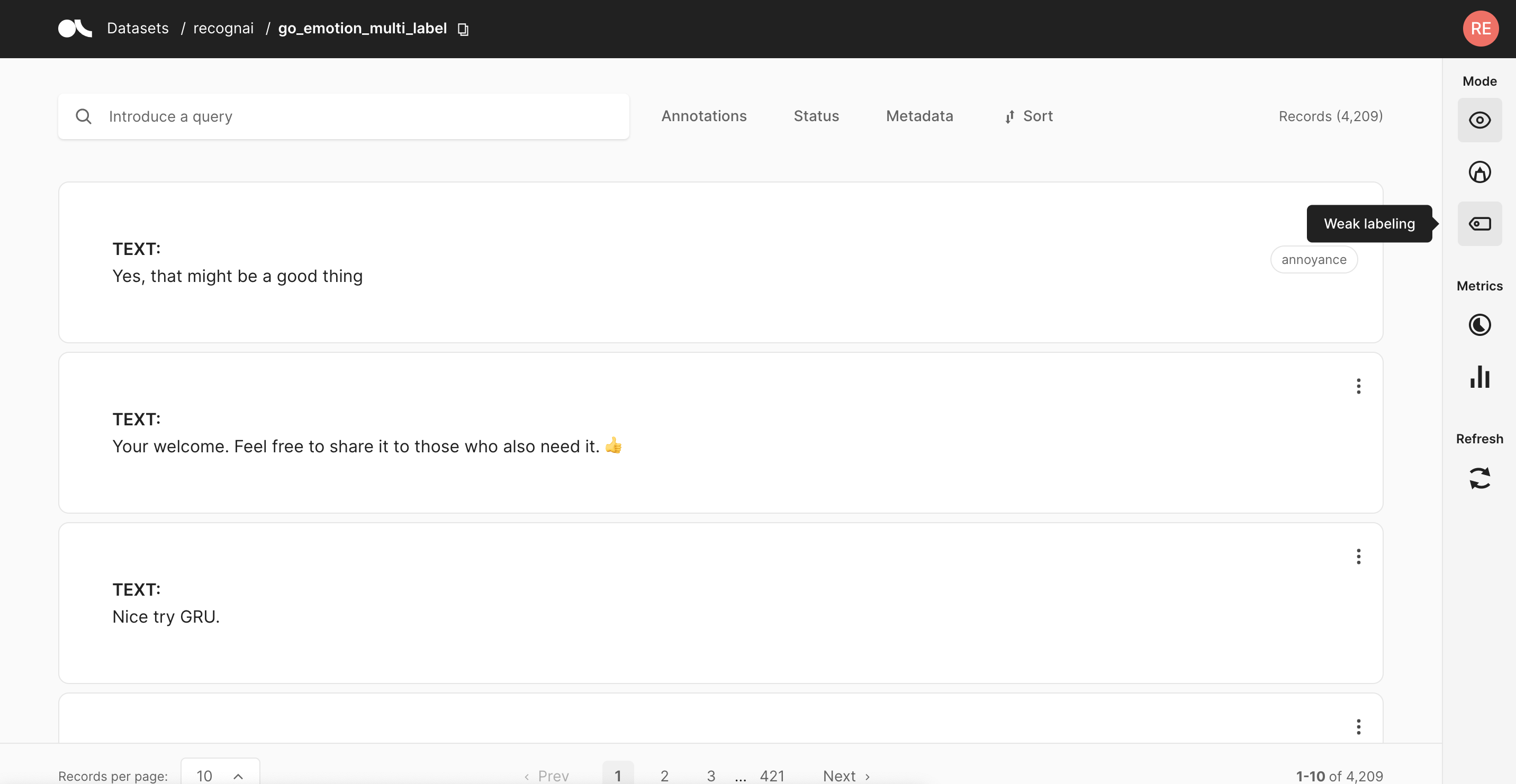
上传数据集后,我们可以探索和检查它以找到好的启发式规则。 为此,我们强烈推荐 Argilla Web 应用程序的专用 定义规则模式,该模式允许您快速迭代启发式规则,计算其指标并保存它们。
在这里,我们将通过 Web 应用程序找到的规则复制到 Notebook 中,以便您轻松地跟随本教程。
[7]:
# Define our heuristic rules, they can surely be improved
rules = [
    Rule("thank*", "gratitude"),
    Rule("appreciate", "gratitude"),
    Rule("text:(thanks AND good)", ["admiration", "gratitude"]),
    Rule("advice", "admiration"),
    Rule("amazing", "admiration"),
    Rule("awesome", "admiration"),
    Rule("impressed", "admiration"),
    Rule("text:(good AND (point OR call OR idea OR job))", "admiration"),
    Rule("legend", "admiration"),
    Rule("exactly", "approval"),
    Rule("agree", "approval"),
    Rule("yeah", "optimism"),
    Rule("suck", "annoyance"),
    Rule("pissed", "annoyance"),
    Rule("annoying", "annoyance"),
    Rule("ruined", "annoyance"),
    Rule("hoping", "optimism"),
    Rule("joking", ["optimism", "admiration"]),
    Rule('text:("good luck")', "optimism"),
    Rule('"nice day"', "optimism"),
    Rule('"what is"', "curiosity"),
    Rule('"can you"', "curiosity"),
    Rule('"would you"', "curiosity"),
    Rule('"do you"', ["curiosity", "admiration"]),
    Rule('"great"', ["annoyance"])
]
我们继续将这些启发式规则应用于我们的数据集,创建我们的弱标签矩阵。 由于我们正在处理多标签分类任务,因此弱标签矩阵将具有 3 个维度。
弱多标签矩阵的维度:记录数 x 规则数 x 标签数
它将填充 0 和 1,具体取决于规则是否对相应标签进行了投票。 如果规则对于给定记录被弃权,则矩阵将填充 -1。
我们可以调用 weak_labels.summary() 方法来检查每个规则的精度以及我们数据集的总覆盖率。
[10]:
# Compute the weak labels for our dataset given the rules.
# If your dataset already contains rules you can omit the rules argument.
add_rules(dataset="go_emotions", rules=rules)
weak_labels = WeakMultiLabels("go_emotions")

# Check coverage/precision of our rules
weak_labels.summary()
[10]:
| 标签 | 覆盖率 | 带注释的覆盖率 | 重叠 | 正确 | 不正确 | 精度 | |
|---|---|---|---|---|---|---|---|
| thank* | {gratitude} | 0.199382 | 0.198925 | 0.048004 | 74 | 0 | 1.000000 |
| appreciate | {gratitude} | 0.016397 | 0.021505 | 0.009981 | 7 | 1 | 0.875000 |
| text:(thanks AND good) | {admiration, gratitude} | 0.007842 | 0.010753 | 0.007842 | 8 | 0 | 1.000000 |
| advice | {admiration} | 0.008317 | 0.008065 | 0.007605 | 3 | 0 | 1.000000 |
| amazing | {admiration} | 0.025428 | 0.021505 | 0.004990 | 8 | 0 | 1.000000 |
| awesome | {admiration} | 0.025190 | 0.034946 | 0.007605 | 12 | 1 | 0.923077 |
| impressed | {admiration} | 0.002139 | 0.005376 | 0.000000 | 2 | 0 | 1.000000 |
| text:(good AND (point OR call OR idea OR job)) | {admiration} | 0.008555 | 0.018817 | 0.003089 | 7 | 0 | 1.000000 |
| legend | {admiration} | 0.001901 | 0.002688 | 0.000475 | 1 | 0 | 1.000000 |
| exactly | {approval} | 0.007842 | 0.010753 | 0.002376 | 3 | 1 | 0.750000 |
| agree | {approval} | 0.016873 | 0.021505 | 0.003327 | 6 | 2 | 0.750000 |
| yeah | {optimism} | 0.024952 | 0.021505 | 0.006179 | 2 | 6 | 0.250000 |
| suck | {annoyance} | 0.002139 | 0.008065 | 0.000475 | 3 | 0 | 1.000000 |
| pissed | {annoyance} | 0.002139 | 0.008065 | 0.000713 | 2 | 1 | 0.666667 |
| annoying | {annoyance} | 0.003327 | 0.018817 | 0.001188 | 7 | 0 | 1.000000 |
| ruined | {annoyance} | 0.000713 | 0.002688 | 0.000238 | 1 | 0 | 1.000000 |
| hoping | {optimism} | 0.003565 | 0.005376 | 0.000713 | 2 | 0 | 1.000000 |
| joking | {admiration, optimism} | 0.000238 | 0.000000 | 0.000000 | 0 | 0 | NaN |
| text:("good luck") | {optimism} | 0.015209 | 0.018817 | 0.002614 | 4 | 3 | 0.571429 |
| "nice day" | {optimism} | 0.000713 | 0.005376 | 0.000000 | 2 | 0 | 1.000000 |
| "what is" | {curiosity} | 0.004040 | 0.005376 | 0.001188 | 2 | 0 | 1.000000 |
| "can you" | {curiosity} | 0.004278 | 0.008065 | 0.000713 | 3 | 0 | 1.000000 |
| "would you" | {curiosity} | 0.000951 | 0.005376 | 0.000238 | 2 | 0 | 1.000000 |
| "do you" | {admiration, curiosity} | 0.010932 | 0.018817 | 0.002376 | 7 | 7 | 0.500000 |
| "great" | {annoyance} | 0.055133 | 0.061828 | 0.016873 | 1 | 22 | 0.043478 |
| total | {approval, gratitude, admiration, optimism, cu... | 0.379753 | 0.448925 | 0.060361 | 169 | 44 | 0.793427 |
我们可以观察到“joking”没有任何支持,并且“do you”也没有信息量,因为它的正确/不正确比率等于 1。 我们可以使用“delete_rules”方法从数据集中删除这两个规则
[13]:
rules_to_delete = [
    Rule("joking", ["optimism", "admiration"]),
    Rule('"do you"', ["curiosity", "admiration"])]

delete_rules(dataset="go_emotions", rules=rules_to_delete)

weak_labels = WeakMultiLabels("go_emotions")
weak_labels.summary()
[13]:
| 标签 | 覆盖率 | 带注释的覆盖率 | 重叠 | 正确 | 不正确 | 精度 | |
|---|---|---|---|---|---|---|---|
| thank* | {gratitude} | 0.199382 | 0.198925 | 0.047766 | 74 | 0 | 1.000000 |
| appreciate | {gratitude} | 0.016397 | 0.021505 | 0.009743 | 7 | 1 | 0.875000 |
| text:(thanks AND good) | {admiration, gratitude} | 0.007842 | 0.010753 | 0.007842 | 8 | 0 | 1.000000 |
| advice | {admiration} | 0.008317 | 0.008065 | 0.007367 | 3 | 0 | 1.000000 |
| amazing | {admiration} | 0.025428 | 0.021505 | 0.004990 | 8 | 0 | 1.000000 |
| awesome | {admiration} | 0.025190 | 0.034946 | 0.007129 | 12 | 1 | 0.923077 |
| impressed | {admiration} | 0.002139 | 0.005376 | 0.000000 | 2 | 0 | 1.000000 |
| text:(good AND (point OR call OR idea OR job)) | {admiration} | 0.008555 | 0.018817 | 0.003089 | 7 | 0 | 1.000000 |
| legend | {admiration} | 0.001901 | 0.002688 | 0.000475 | 1 | 0 | 1.000000 |
| exactly | {approval} | 0.007842 | 0.010753 | 0.002139 | 3 | 1 | 0.750000 |
| agree | {approval} | 0.016873 | 0.021505 | 0.003327 | 6 | 2 | 0.750000 |
| yeah | {optimism} | 0.024952 | 0.021505 | 0.006179 | 2 | 6 | 0.250000 |
| suck | {annoyance} | 0.002139 | 0.008065 | 0.000475 | 3 | 0 | 1.000000 |
| pissed | {annoyance} | 0.002139 | 0.008065 | 0.000475 | 2 | 1 | 0.666667 |
| annoying | {annoyance} | 0.003327 | 0.018817 | 0.001188 | 7 | 0 | 1.000000 |
| ruined | {annoyance} | 0.000713 | 0.002688 | 0.000238 | 1 | 0 | 1.000000 |
| hoping | {optimism} | 0.003565 | 0.005376 | 0.000713 | 2 | 0 | 1.000000 |
| text:("good luck") | {optimism} | 0.015209 | 0.018817 | 0.002614 | 4 | 3 | 0.571429 |
| "nice day" | {optimism} | 0.000713 | 0.005376 | 0.000000 | 2 | 0 | 1.000000 |
| "what is" | {curiosity} | 0.004040 | 0.005376 | 0.001188 | 2 | 0 | 1.000000 |
| "can you" | {curiosity} | 0.004278 | 0.008065 | 0.000713 | 3 | 0 | 1.000000 |
| "would you" | {curiosity} | 0.000951 | 0.005376 | 0.000238 | 2 | 0 | 1.000000 |
| "great" | {annoyance} | 0.055133 | 0.061828 | 0.016397 | 1 | 22 | 0.043478 |
| total | {approval, gratitude, admiration, optimism, cu... | 0.370960 | 0.435484 | 0.058222 | 162 | 37 | 0.814070 |
我们可以观察到以下规则效果不佳;
Rule('"great"', ["annoyance"])

Rule("yeah", "optimism"),
让我们更新这两个规则,例如
Rule('"great"', ["admiration"])

Rule("yeah", "approval"),
[14]:
rules_to_update = [
    Rule('"great"', ["admiration"]),
    Rule("yeah", "approval")]

update_rules(dataset="go_emotions", rules=rules_to_update)
让我们使用数据集的最终规则运行弱标签
[17]:
weak_labels = WeakMultiLabels(dataset="go_emotions")
weak_labels.summary()
[17]:
| 标签 | 覆盖率 | 带注释的覆盖率 | 重叠 | 正确 | 不正确 | 精度 | |
|---|---|---|---|---|---|---|---|
| thank* | {gratitude} | 0.199382 | 0.198925 | 0.047766 | 74 | 0 | 1.000000 |
| appreciate | {gratitude} | 0.016397 | 0.021505 | 0.009743 | 7 | 1 | 0.875000 |
| text:(thanks AND good) | {admiration, gratitude} | 0.007842 | 0.010753 | 0.007842 | 8 | 0 | 1.000000 |
| advice | {admiration} | 0.008317 | 0.008065 | 0.007367 | 3 | 0 | 1.000000 |
| amazing | {admiration} | 0.025428 | 0.021505 | 0.004990 | 8 | 0 | 1.000000 |
| awesome | {admiration} | 0.025190 | 0.034946 | 0.007129 | 12 | 1 | 0.923077 |
| impressed | {admiration} | 0.002139 | 0.005376 | 0.000000 | 2 | 0 | 1.000000 |
| text:(good AND (point OR call OR idea OR job)) | {admiration} | 0.008555 | 0.018817 | 0.003089 | 7 | 0 | 1.000000 |
| legend | {admiration} | 0.001901 | 0.002688 | 0.000475 | 1 | 0 | 1.000000 |
| exactly | {approval} | 0.007842 | 0.010753 | 0.002139 | 3 | 1 | 0.750000 |
| agree | {approval} | 0.016873 | 0.021505 | 0.003327 | 6 | 2 | 0.750000 |
| yeah | {approval} | 0.024952 | 0.021505 | 0.006179 | 5 | 3 | 0.625000 |
| suck | {annoyance} | 0.002139 | 0.008065 | 0.000475 | 3 | 0 | 1.000000 |
| pissed | {annoyance} | 0.002139 | 0.008065 | 0.000475 | 2 | 1 | 0.666667 |
| annoying | {annoyance} | 0.003327 | 0.018817 | 0.001188 | 7 | 0 | 1.000000 |
| ruined | {annoyance} | 0.000713 | 0.002688 | 0.000238 | 1 | 0 | 1.000000 |
| hoping | {optimism} | 0.003565 | 0.005376 | 0.000713 | 2 | 0 | 1.000000 |
| text:("good luck") | {optimism} | 0.015209 | 0.018817 | 0.002614 | 4 | 3 | 0.571429 |
| "nice day" | {optimism} | 0.000713 | 0.005376 | 0.000000 | 2 | 0 | 1.000000 |
| "what is" | {curiosity} | 0.004040 | 0.005376 | 0.001188 | 2 | 0 | 1.000000 |
| "can you" | {curiosity} | 0.004278 | 0.008065 | 0.000713 | 3 | 0 | 1.000000 |
| "would you" | {curiosity} | 0.000951 | 0.005376 | 0.000238 | 2 | 0 | 1.000000 |
| "great" | {admiration} | 0.055133 | 0.061828 | 0.016397 | 19 | 4 | 0.826087 |
| total | {approval, gratitude, admiration, optimism, cu... | 0.370960 | 0.435484 | 0.058222 | 183 | 16 | 0.919598 |
让我们考虑一下我们想要尝试一个规则
[20]:
optimism_rule = Rule("wish*", "optimism")
optimism_rule.apply(dataset="go_emotions")
optimism_rule.metrics(dataset="go_emotions")
[20]:
{'coverage': 0.006178707224334601,
 'annotated_coverage': 0.0,
 'correct': 0,
 'incorrect': 0,
 'precision': None}
optimism_rule 没有信息量,所以我们不将其添加到数据集中
让我们尝试一个 curiosity 类的规则
[23]:
curiosity_rule = Rule("could you", "curiosity")
curiosity_rule.apply("go_emotions")
curiosity_rule.metrics(dataset="go_emotions")
[23]:
{'coverage': 0.005465779467680608,
 'annotated_coverage': 0.002688172043010753,
 'correct': 1,
 'incorrect': 0,
 'precision': 1.0}
curiosity_rule 具有积极的支持,我们可以按如下方式将其添加到数据集中
[24]:
curiosity_rule.add_to_dataset(dataset="go_emotions")
让我们使用最终规则集再次应用弱标签
[26]:
weak_labels = WeakMultiLabels(dataset="go_emotions")
weak_labels.summary()
[26]:
| 标签 | 覆盖率 | 带注释的覆盖率 | 重叠 | 正确 | 不正确 | 精度 | |
|---|---|---|---|---|---|---|---|
| thank* | {gratitude} | 0.199382 | 0.198925 | 0.048004 | 74 | 0 | 1.000000 |
| appreciate | {gratitude} | 0.016397 | 0.021505 | 0.009743 | 7 | 1 | 0.875000 |
| text:(thanks AND good) | {admiration, gratitude} | 0.007842 | 0.010753 | 0.007842 | 8 | 0 | 1.000000 |
| advice | {admiration} | 0.008317 | 0.008065 | 0.007367 | 3 | 0 | 1.000000 |
| amazing | {admiration} | 0.025428 | 0.021505 | 0.004990 | 8 | 0 | 1.000000 |
| awesome | {admiration} | 0.025190 | 0.034946 | 0.007367 | 12 | 1 | 0.923077 |
| impressed | {admiration} | 0.002139 | 0.005376 | 0.000000 | 2 | 0 | 1.000000 |
| text:(good AND (point OR call OR idea OR job)) | {admiration} | 0.008555 | 0.018817 | 0.003089 | 7 | 0 | 1.000000 |
| legend | {admiration} | 0.001901 | 0.002688 | 0.000475 | 1 | 0 | 1.000000 |
| exactly | {approval} | 0.007842 | 0.010753 | 0.002139 | 3 | 1 | 0.750000 |
| agree | {approval} | 0.016873 | 0.021505 | 0.003565 | 6 | 2 | 0.750000 |
| yeah | {approval} | 0.024952 | 0.021505 | 0.006179 | 5 | 3 | 0.625000 |
| suck | {annoyance} | 0.002139 | 0.008065 | 0.000475 | 3 | 0 | 1.000000 |
| pissed | {annoyance} | 0.002139 | 0.008065 | 0.000475 | 2 | 1 | 0.666667 |
| annoying | {annoyance} | 0.003327 | 0.018817 | 0.001188 | 7 | 0 | 1.000000 |
| ruined | {annoyance} | 0.000713 | 0.002688 | 0.000238 | 1 | 0 | 1.000000 |
| hoping | {optimism} | 0.003565 | 0.005376 | 0.000713 | 2 | 0 | 1.000000 |
| text:("good luck") | {optimism} | 0.015209 | 0.018817 | 0.002614 | 4 | 3 | 0.571429 |
| "nice day" | {optimism} | 0.000713 | 0.005376 | 0.000000 | 2 | 0 | 1.000000 |
| "what is" | {curiosity} | 0.004040 | 0.005376 | 0.001188 | 2 | 0 | 1.000000 |
| "can you" | {curiosity} | 0.004278 | 0.008065 | 0.000713 | 3 | 0 | 1.000000 |
| "would you" | {curiosity} | 0.000951 | 0.005376 | 0.000475 | 2 | 0 | 1.000000 |
| "great" | {admiration} | 0.055133 | 0.061828 | 0.016397 | 19 | 4 | 0.826087 |
| could you | {curiosity} | 0.005466 | 0.002688 | 0.001188 | 1 | 0 | 1.000000 |
| total | {approval, gratitude, admiration, optimism, cu... | 0.375238 | 0.435484 | 0.059173 | 184 | 16 | 0.920000 |
创建训练集#
当我们对启发式方法感到满意时,就该将它们组合起来并计算弱标签,以便训练我们的下游模型。 为此,我们将使用 MajorityVoter。 在多标签情况下,它将标签的概率设置为 0 或 1,具体取决于是否至少有一个非弃权规则对相应标签进行了投票。
[ ]:
# Use the majority voter as the label model
label_model = MajorityVoter(weak_labels)
从我们的标签模型中,我们获得了训练记录及其弱标签和概率。 我们将使用概率大于 0.5 的弱标签作为我们训练的标签,因此将它们复制到我们记录的 annotation 属性中。
[ ]:
# Get records with the predictions from the label model to train a down-stream model
train_rg = label_model.predict()

# Copy label model predictions to annotation with a threshold of 0.5
for rec in train_rg:
    rec.annotation = [pred[0] for pred in rec.prediction if pred[1] > 0.5]
我们从 WeakMultiLabels 对象中提取带有手动注释的测试集
[ ]:
# Get records with manual annotations to use as test set for the down-stream model
test_rg = rg.DatasetForTextClassification(weak_labels.records(has_annotation=True))
我们将使用方便的 DatasetForTextClassification.prepare_for_training() 方法来创建针对使用 Hugging Face transformers 库进行训练而优化的数据集
[ ]:
from datasets import DatasetDict

# Create dataset dictionary and shuffle training set
ds = DatasetDict(
    train=train_rg.prepare_for_training().shuffle(seed=42),
    test=test_rg.prepare_for_training(),
)
训练 Transformer 下游模型#
以下步骤基本上是从 Hugging Face transformers 库的精彩文档中复制和粘贴的。
首先,我们将加载与我们的模型相对应的 tokenizer,我们选择它是臭名昭著的 BERT 的 精馏版本。
注意
由于我们将使用功能齐全的 Transformer 作为下游模型(尽管是精馏的),因此我们建议在具有 GPU 的机器上或在启用 GPU 后端的 Google Colab 中执行以下代码。
[ ]:
from transformers import AutoTokenizer

# Initialize tokenizer
tokenizer = AutoTokenizer.from_pretrained("distilbert-base-uncased")
之后,我们标记化我们的数据
[ ]:
def tokenize_func(examples):
    return tokenizer(examples["text"], padding="max_length", truncation=True)


# Tokenize the data
tokenized_ds = ds.map(tokenize_func, batched=True)
Transformer 模型期望我们的标签遵循通用的二进制多标签格式,因此让我们使用 sklearn 进行此转换。
[ ]:
from sklearn.preprocessing import MultiLabelBinarizer

# Turn labels into multi-label format
mb = MultiLabelBinarizer()
mb.fit(ds["test"]["label"])


def binarize_labels(examples):
    return {"label": mb.transform(examples["label"])}


binarized_tokenized_ds = tokenized_ds.map(binarize_labels, batched=True)
在我们开始训练之前,定义我们的评估指标非常重要。 在这里,我们选择了常用的微平均 F1 指标,但我们还将跟踪 每个标签的 F1,以便之后进行更深入的错误分析。
[ ]:
from datasets import load_metric
import numpy as np

# Define our metrics
metric = load_metric("f1", config_name="multilabel")


def compute_metrics(eval_pred):
    logits, labels = eval_pred
    # apply sigmoid
    predictions = (1.0 / (1 + np.exp(-logits))) > 0.5

    # f1 micro averaged
    metrics = metric.compute(
        predictions=predictions, references=labels, average="micro"
    )
    # f1 per label
    per_label_metric = metric.compute(
        predictions=predictions, references=labels, average=None
    )
    for label, f1 in zip(
        ds["train"].features["label"][0].names, per_label_metric["f1"]
    ):
        metrics[f"f1_{label}"] = f1

    return metrics
现在我们准备好加载我们的预训练 Transformer 模型,并为我们的任务做好准备:具有 6 个标签的多标签文本分类。
[ ]:
from transformers import AutoModelForSequenceClassification

# Init our down-stream model
model = AutoModelForSequenceClassification.from_pretrained(
    "distilbert-base-uncased", problem_type="multi_label_classification", num_labels=6
)
训练中唯一缺少的是 Trainer 及其 TrainingArguments。 为了简单起见,我们主要依赖默认参数,这些参数通常开箱即用,但稍微调整了批处理大小以加快训练速度。 我们还检查了 2 个 epoch 对于我们相当小的数据集来说已经足够了。
[ ]:
from transformers import TrainingArguments

# Set our training arguments
training_args = TrainingArguments(
    output_dir="test_trainer",
    evaluation_strategy="epoch",
    num_train_epochs=2,
    per_device_train_batch_size=16,
    per_device_eval_batch_size=16,
)
[ ]:
from transformers import Trainer

# Init the trainer
trainer = Trainer(
    model=model,
    args=training_args,
    train_dataset=binarized_tokenized_ds["train"],
    eval_dataset=binarized_tokenized_ds["test"],
    compute_metrics=compute_metrics,
)
[ ]:
# Train the down-stream model
trainer.train()
我们实现了约 0.54 的微平均 F1,这并不完美,但对于这个具有挑战性的数据集来说是一个很好的基线。 当检查每个标签的 F1 时,我们清楚地看到,性能最差的标签是在准确性和覆盖率方面启发式方法最差的标签,这不足为奇。
研究主题数据集#
在介绍了多标签情感分类任务之后,我们将尝试对与主题建模相关的多标签分类任务执行相同的操作。 在此数据集中,研究论文根据其标题和摘要分为 6 个非独占标签。
我们将尝试仅根据标题对论文进行分类,这相当困难,但允许我们快速浏览数据并提出启发式方法。 有关最少数据预处理的所有详细信息,请参见附录 B。
定义规则#
让我们首先从 Hugging Face Hub 下载我们预处理的数据集,并将其记录到 Argilla
[ ]:
# Download preprocessed dataset
ds_rb = rg.read_datasets(
    load_dataset("argilla/research_titles_multi-label", split="train"),
    task="TextClassification",
)
[ ]:
# Log dataset to Argilla to find good heuristics
rg.log(ds_rb, "research_titles")
上传数据集后,我们可以探索和检查它以找到好的启发式规则。 为此,我们强烈推荐 Argilla Web 应用程序的专用 定义规则模式,它允许您快速迭代启发式规则,计算其指标并保存它们。
在这里,我们将通过 Web 应用程序找到的规则复制到 Notebook 中,以便您轻松地跟随本教程。
[29]:
# Define our heuristic rules (can probably be improved)
rules = [
    Rule("stock*", "Quantitative Finance"),
    Rule("*asset*", "Quantitative Finance"),
    Rule("pric*", "Quantitative Finance"),
    Rule("economy", "Quantitative Finance"),
    Rule("deep AND neural AND network*", "Computer Science"),
    Rule("convolutional", "Computer Science"),
    Rule("allocat* AND *net*", "Computer Science"),
    Rule("program", "Computer Science"),
    Rule("classification* AND (label* OR deep)", "Computer Science"),
    Rule("scattering", "Physics"),
    Rule("astro*", "Physics"),
    Rule("optical", "Physics"),
    Rule("ray", "Physics"),
    Rule("entangle*", "Physics"),
    Rule("*algebra*", "Mathematics"),
    Rule("spaces", "Mathematics"),
    Rule("operators", "Mathematics"),
    Rule("estimation", "Statistics"),
    Rule("mixture", "Statistics"),
    Rule("gaussian", "Statistics"),
    Rule("gene", "Quantitative Biology"),
]
我们继续将这些启发式规则应用于我们的数据集,创建我们的弱标签矩阵。 如 GoEmotions 部分所述,弱标签矩阵将具有 3 个维度和 -1、0 和 1 的值。
让我们概述一下我们的启发式方法以及它们的性能
[31]:
# Compute the weak labels for our dataset given the rules
# If your dataset already contains rules you can omit the rules argument.
add_rules(dataset="research_titles", rules=rules)
weak_labels = WeakMultiLabels("research_titles")
weak_labels.summary()
[31]:
| 标签 | 覆盖率 | 带注释的覆盖率 | 重叠 | 正确 | 不正确 | 精度 | |
|---|---|---|---|---|---|---|---|
| stock* | {Quantitative Finance} | 0.000954 | 0.000715 | 0.000191 | 3 | 0 | 1.000000 |
| *asset* | {Quantitative Finance} | 0.000477 | 0.000715 | 0.000238 | 3 | 0 | 1.000000 |
| pric* | {Quantitative Finance} | 0.003433 | 0.003337 | 0.000668 | 9 | 5 | 0.642857 |
| economy | {Quantitative Finance} | 0.000238 | 0.000238 | 0.000000 | 1 | 0 | 1.000000 |
| deep AND neural AND network* | {Computer Science} | 0.009155 | 0.010250 | 0.002575 | 32 | 11 | 0.744186 |
| convolutional | {Computer Science} | 0.010109 | 0.009297 | 0.002003 | 32 | 7 | 0.820513 |
| allocat* AND *net* | {Computer Science} | 0.000763 | 0.000715 | 0.000000 | 3 | 0 | 1.000000 |
| program | {Computer Science} | 0.002623 | 0.003099 | 0.000095 | 11 | 2 | 0.846154 |
| classification* AND (label* OR deep) | {Computer Science} | 0.003338 | 0.004052 | 0.001287 | 14 | 3 | 0.823529 |
| scattering | {Physics} | 0.004053 | 0.002861 | 0.000572 | 10 | 2 | 0.833333 |
| astro* | {Physics} | 0.003099 | 0.004052 | 0.000477 | 17 | 0 | 1.000000 |
| optical | {Physics} | 0.007105 | 0.006913 | 0.000811 | 27 | 2 | 0.931034 |
| ray | {Physics} | 0.005865 | 0.007390 | 0.000668 | 27 | 4 | 0.870968 |
| entangle* | {Physics} | 0.002623 | 0.002861 | 0.000048 | 11 | 1 | 0.916667 |
| *algebra* | {Mathematics} | 0.014829 | 0.018355 | 0.000429 | 70 | 7 | 0.909091 |
| spaces | {Mathematics} | 0.010586 | 0.009774 | 0.001287 | 38 | 3 | 0.926829 |
| operators | {Mathematics} | 0.006151 | 0.005959 | 0.001192 | 22 | 3 | 0.880000 |
| estimation | {Statistics} | 0.021266 | 0.021216 | 0.001621 | 65 | 24 | 0.730337 |
| mixture | {Statistics} | 0.003290 | 0.003099 | 0.000906 | 10 | 3 | 0.769231 |
| gaussian | {Statistics} | 0.009250 | 0.011204 | 0.001526 | 36 | 11 | 0.765957 |
| gene | {Quantitative Biology} | 0.001287 | 0.001669 | 0.000143 | 6 | 1 | 0.857143 |
| total | {Mathematics, Quantitative Biology, Physics, Q... | 0.111911 | 0.118951 | 0.008154 | 447 | 89 | 0.833955 |
考虑一下我们提出了新规则并想将它们添加到数据集中的情况
[32]:
additional_rules = [
    Rule("trading", "Quantitative Finance"),
    Rule("finance", "Quantitative Finance"),
    Rule("memor* AND (design* OR network*)", "Computer Science"),
    Rule("system* AND design*", "Computer Science"),
    Rule("material*", "Physics"),
    Rule("spin", "Physics"),
    Rule("magnetic", "Physics"),
    Rule("manifold* AND (NOT learn*)", "Mathematics"),
    Rule("equation", "Mathematics"),
    Rule("regression", "Statistics"),
    Rule("bayes*", "Statistics"),
]
[35]:
add_rules(dataset="research_titles", rules=additional_rules)
weak_labels = WeakMultiLabels("research_titles")
weak_labels.summary()
[35]:
| 标签 | 覆盖率 | 带注释的覆盖率 | 重叠 | 正确 | 不正确 | 精度 | |
|---|---|---|---|---|---|---|---|
| stock* | {Quantitative Finance} | 0.000954 | 0.000715 | 0.000334 | 3 | 0 | 1.000000 |
| *asset* | {Quantitative Finance} | 0.000477 | 0.000715 | 0.000286 | 3 | 0 | 1.000000 |
| pric* | {Quantitative Finance} | 0.003433 | 0.003337 | 0.000715 | 9 | 5 | 0.642857 |
| economy | {Quantitative Finance} | 0.000238 | 0.000238 | 0.000000 | 1 | 0 | 1.000000 |
| deep AND neural AND network* | {Computer Science} | 0.009155 | 0.010250 | 0.002909 | 32 | 11 | 0.744186 |
| convolutional | {Computer Science} | 0.010109 | 0.009297 | 0.002241 | 32 | 7 | 0.820513 |
| allocat* AND *net* | {Computer Science} | 0.000763 | 0.000715 | 0.000000 | 3 | 0 | 1.000000 |
| program | {Computer Science} | 0.002623 | 0.003099 | 0.000143 | 11 | 2 | 0.846154 |
| classification* AND (label* OR deep) | {Computer Science} | 0.003338 | 0.004052 | 0.001335 | 14 | 3 | 0.823529 |
| scattering | {Physics} | 0.004053 | 0.002861 | 0.001001 | 10 | 2 | 0.833333 |
| astro* | {Physics} | 0.003099 | 0.004052 | 0.000620 | 17 | 0 | 1.000000 |
| optical | {Physics} | 0.007105 | 0.006913 | 0.001097 | 27 | 2 | 0.931034 |
| ray | {Physics} | 0.005865 | 0.007390 | 0.001192 | 27 | 4 | 0.870968 |
| entangle* | {Physics} | 0.002623 | 0.002861 | 0.000095 | 11 | 1 | 0.916667 |
| *algebra* | {Mathematics} | 0.014829 | 0.018355 | 0.000620 | 70 | 7 | 0.909091 |
| spaces | {Mathematics} | 0.010586 | 0.009774 | 0.001860 | 38 | 3 | 0.926829 |
| operators | {Mathematics} | 0.006151 | 0.005959 | 0.001526 | 22 | 3 | 0.880000 |
| estimation | {Statistics} | 0.021266 | 0.021216 | 0.003385 | 65 | 24 | 0.730337 |
| mixture | {Statistics} | 0.003290 | 0.003099 | 0.001287 | 10 | 3 | 0.769231 |
| gaussian | {Statistics} | 0.009250 | 0.011204 | 0.002766 | 36 | 11 | 0.765957 |
| gene | {Quantitative Biology} | 0.001287 | 0.001669 | 0.000191 | 6 | 1 | 0.857143 |
| trading | {Quantitative Finance} | 0.000954 | 0.000238 | 0.000191 | 1 | 0 | 1.000000 |
| finance | {Quantitative Finance} | 0.000048 | 0.000238 | 0.000000 | 1 | 0 | 1.000000 |
| memor* AND (design* OR network*) | {Computer Science} | 0.001383 | 0.002145 | 0.000286 | 9 | 0 | 1.000000 |
| system* AND design* | {Computer Science} | 0.001144 | 0.002384 | 0.000238 | 9 | 1 | 0.900000 |
| material* | {Physics} | 0.004148 | 0.003099 | 0.000238 | 10 | 3 | 0.769231 |
| spin | {Physics} | 0.013542 | 0.015018 | 0.002146 | 60 | 3 | 0.952381 |
| magnetic | {Physics} | 0.011301 | 0.012872 | 0.002432 | 49 | 5 | 0.907407 |
| manifold* AND (NOT learn*) | {Mathematics} | 0.007057 | 0.008343 | 0.000858 | 28 | 7 | 0.800000 |
| equation | {Mathematics} | 0.010681 | 0.007867 | 0.000954 | 24 | 9 | 0.727273 |
| regression | {Statistics} | 0.009393 | 0.009058 | 0.002575 | 33 | 5 | 0.868421 |
| bayes* | {Statistics} | 0.015306 | 0.014779 | 0.003147 | 49 | 13 | 0.790323 |
| total | {Mathematics, Quantitative Biology, Physics, Q... | 0.176616 | 0.185936 | 0.017833 | 720 | 135 | 0.842105 |
让我们创建新规则并查看其效果,如果它们信息量足够,我们可以继续将它们添加到数据集中
[36]:
# create a statistics rule and get its metrics
statistics_rule = Rule("sample", "Statistics")
statistics_rule.apply("research_titles")
statistics_rule.metrics("research_titles")
[36]:
{'coverage': 0.004672897196261682,
 'annotated_coverage': 0.004529201430274136,
 'correct': 17,
 'incorrect': 2,
 'precision': 0.8947368421052632}
[37]:
# add the statistics_rule to the research_titles dataset
statistics_rule.add_to_dataset("research_titles")
[38]:
finance_rule = Rule("risk", "Quantitative Finance")
finance_rule.apply("research_titles")
finance_rule.metrics("research_titles")
[38]:
{'coverage': 0.004815945069616631,
 'annotated_coverage': 0.004290822407628129,
 'correct': 1,
 'incorrect': 17,
 'precision': 0.05555555555555555}
[39]:
finance_rule.add_to_dataset("research_titles")
我们的断言似乎不正确,让我们更新此规则
[40]:
rule = Rule("risk", "Statistics")
[41]:
rule.metrics("research_titles")
[41]:
{'coverage': 0.004815945069616631,
 'annotated_coverage': 0.004290822407628129,
 'correct': 11,
 'incorrect': 7,
 'precision': 0.6111111111111112}
[42]:
rule.update_at_dataset("research_titles")
[43]:
quantitative_biology_rule = Rule("dna", "Quantitative Biology")
[44]:
quantitative_biology_rule.metrics("research_titles")
[44]:
{'coverage': 0.0013351134846461949,
 'annotated_coverage': 0.0011918951132300357,
 'correct': 4,
 'incorrect': 1,
 'precision': 0.8}
[45]:
quantitative_biology_rule.add_to_dataset("research_titles")
让我们看看包含新添加规则的最终矩阵
[47]:
weak_labels = WeakMultiLabels("research_titles")
weak_labels.summary()
[47]:
| 标签 | 覆盖率 | 带注释的覆盖率 | 重叠 | 正确 | 不正确 | 精度 | |
|---|---|---|---|---|---|---|---|
| stock* | {Quantitative Finance} | 0.000954 | 0.000715 | 0.000334 | 3 | 0 | 1.000000 |
| *asset* | {Quantitative Finance} | 0.000477 | 0.000715 | 0.000334 | 3 | 0 | 1.000000 |
| pric* | {Quantitative Finance} | 0.003433 | 0.003337 | 0.000811 | 9 | 5 | 0.642857 |
| economy | {Quantitative Finance} | 0.000238 | 0.000238 | 0.000048 | 1 | 0 | 1.000000 |
| deep AND neural AND network* | {Computer Science} | 0.009155 | 0.010250 | 0.002956 | 32 | 11 | 0.744186 |
| convolutional | {Computer Science} | 0.010109 | 0.009297 | 0.002336 | 32 | 7 | 0.820513 |
| allocat* AND *net* | {Computer Science} | 0.000763 | 0.000715 | 0.000048 | 3 | 0 | 1.000000 |
| program | {Computer Science} | 0.002623 | 0.003099 | 0.000191 | 11 | 2 | 0.846154 |
| classification* AND (label* OR deep) | {Computer Science} | 0.003338 | 0.004052 | 0.001335 | 14 | 3 | 0.823529 |
| scattering | {Physics} | 0.004053 | 0.002861 | 0.001049 | 10 | 2 | 0.833333 |
| astro* | {Physics} | 0.003099 | 0.004052 | 0.000668 | 17 | 0 | 1.000000 |
| optical | {Physics} | 0.007105 | 0.006913 | 0.001097 | 27 | 2 | 0.931034 |
| ray | {Physics} | 0.005865 | 0.007390 | 0.001240 | 27 | 4 | 0.870968 |
| entangle* | {Physics} | 0.002623 | 0.002861 | 0.000095 | 11 | 1 | 0.916667 |
| *algebra* | {Mathematics} | 0.014829 | 0.018355 | 0.000620 | 70 | 7 | 0.909091 |
| spaces | {Mathematics} | 0.010586 | 0.009774 | 0.001860 | 38 | 3 | 0.926829 |
| operators | {Mathematics} | 0.006151 | 0.005959 | 0.001574 | 22 | 3 | 0.880000 |
| estimation | {Statistics} | 0.021266 | 0.021216 | 0.003862 | 65 | 24 | 0.730337 |
| mixture | {Statistics} | 0.003290 | 0.003099 | 0.001335 | 10 | 3 | 0.769231 |
| gaussian | {Statistics} | 0.009250 | 0.011204 | 0.003052 | 36 | 11 | 0.765957 |
| gene | {Quantitative Biology} | 0.001287 | 0.001669 | 0.000191 | 6 | 1 | 0.857143 |
| trading | {Quantitative Finance} | 0.000954 | 0.000238 | 0.000191 | 1 | 0 | 1.000000 |
| finance | {Quantitative Finance} | 0.000048 | 0.000238 | 0.000000 | 1 | 0 | 1.000000 |
| memor* AND (design* OR network*) | {Computer Science} | 0.001383 | 0.002145 | 0.000286 | 9 | 0 | 1.000000 |
| system* AND design* | {Computer Science} | 0.001144 | 0.002384 | 0.000238 | 9 | 1 | 0.900000 |
| material* | {Physics} | 0.004148 | 0.003099 | 0.000238 | 10 | 3 | 0.769231 |
| spin | {Physics} | 0.013542 | 0.015018 | 0.002146 | 60 | 3 | 0.952381 |
| magnetic | {Physics} | 0.011301 | 0.012872 | 0.002432 | 49 | 5 | 0.907407 |
| manifold* AND (NOT learn*) | {Mathematics} | 0.007057 | 0.008343 | 0.000858 | 28 | 7 | 0.800000 |
| equation | {Mathematics} | 0.010681 | 0.007867 | 0.001001 | 24 | 9 | 0.727273 |
| regression | {Statistics} | 0.009393 | 0.009058 | 0.002718 | 33 | 5 | 0.868421 |
| bayes* | {Statistics} | 0.015306 | 0.014779 | 0.003481 | 49 | 13 | 0.790323 |
| sample | {Statistics} | 0.004673 | 0.004529 | 0.000811 | 17 | 2 | 0.894737 |
| risk | {Statistics} | 0.004816 | 0.004291 | 0.001097 | 11 | 7 | 0.611111 |
| dna | {Quantitative Biology} | 0.001335 | 0.001192 | 0.000143 | 4 | 1 | 0.800000 |
| total | {Mathematics, Quantitative Biology, Physics, Q... | 0.185390 | 0.194041 | 0.019788 | 752 | 145 | 0.838350 |
创建训练集#
当我们对启发式方法感到满意时,就该将它们组合起来并计算弱标签,以便训练我们的下游模型。 对于“GoEmotions”数据集,我们将使用简单的 MajorityVoter。
[48]:
# Use the majority voter as the label model
label_model = MajorityVoter(weak_labels)
从我们的标签模型中,我们获得了训练记录及其弱标签和概率。 由于我们将训练 sklearn 模型,因此我们将记录放入 pandas DataFrame 中,该 DataFrame 通常与 sklearn 生态系统具有良好的集成。
[49]:
train_df = label_model.predict().to_pandas()
在训练我们的模型之前,我们需要从标签模型预测中提取训练标签,并将它们转换为多标签兼容格式。
[50]:
# Create labels in multi-label format, we will use a threshold of 0.5 for the probability
def multi_label_binarizer(predictions, threshold=0.5):
    predicted_labels = [label for label, prob in predictions if prob > threshold]
    binary_labels = [
        1 if label in predicted_labels else 0 for label in weak_labels.labels
    ]
    return binary_labels


train_df["label"] = train_df.prediction.map(multi_label_binarizer)
现在,让我们定义我们的下游模型并对其进行训练。
我们将使用 scikit-multilearn 库来包装多项式 朴素贝叶斯分类器,该分类器适用于具有离散特征的分类(例如,文本分类的字数)。 BinaryRelevance 类将具有 L 个标签的多标签问题转换为 L 个单标签二元分类问题,因此最后我们将自动将 L 个朴素贝叶斯分类器拟合到我们的数据。
我们分类器的特征将是不同单词 n-gram 的计数:也就是说,对于每个示例,我们计算连续 n 个单词的序列数,其中 n 从 1 到 5。 我们使用 CountVectorizer 提取这些特征。
最后,我们将我们的特征提取器和多标签分类器放入 sklearn 管道中,这使得拟合和评分模型变得轻而易举。
[51]:
from skmultilearn.problem_transform import BinaryRelevance
from sklearn.feature_extraction.text import CountVectorizer
from sklearn.naive_bayes import MultinomialNB
from sklearn.pipeline import Pipeline

# Define our down-stream model
classifier = Pipeline(
    [("vect", CountVectorizer()), ("clf", BinaryRelevance(MultinomialNB()))]
)
训练模型就像在我们的管道上调用 fit 方法,并提供我们的训练文本和训练标签一样简单。
[52]:
import numpy as np

# Fit the down-stream classifier
classifier.fit(
    X=train_df.text,
    y=np.array(train_df.label.tolist()),
)
[52]:
Pipeline(steps=[('vect', CountVectorizer()),
                ('clf',
                 BinaryRelevance(classifier=MultinomialNB(),
                                 require_dense=[True, True]))])
在 Jupyter 环境中,请重新运行此单元格以显示 HTML 表示形式或信任 Notebook。在 GitHub 上,HTML 表示形式无法呈现,请尝试使用 nbviewer.org 加载此页面。
Pipeline(steps=[('vect', CountVectorizer()),
                ('clf',
                 BinaryRelevance(classifier=MultinomialNB(),
require_dense=[True, True]))])CountVectorizer()
BinaryRelevance(classifier=MultinomialNB(), require_dense=[True, True])
MultinomialNB()
MultinomialNB()
为了对我们训练的模型进行评分,我们检索其对测试集的预测,并使用 sklearn 的 classification_report 以获得格式良好的字符串中的所有重要分类指标。
[53]:
# Get predictions for test set
predictions = classifier.predict(
    X=[rec.text for rec in weak_labels.records(has_annotation=True)]
)
[54]:
from sklearn.metrics import classification_report

# Compute metrics
print(
    classification_report(
        weak_labels.annotation(), predictions, target_names=weak_labels.labels
    )
)
                      precision    recall  f1-score   support

    Computer Science       0.81      0.24      0.38      1740
         Mathematics       0.79      0.58      0.67      1141
             Physics       0.88      0.65      0.74      1186
Quantitative Biology       0.67      0.02      0.04       109
Quantitative Finance       0.46      0.13      0.21        45
          Statistics       0.52      0.69      0.60      1069

           micro avg       0.71      0.49      0.58      5290
           macro avg       0.69      0.39      0.44      5290
        weighted avg       0.76      0.49      0.56      5290
         samples avg       0.58      0.52      0.53      5290
我们获得了大约 0.59 的微平均 F1 分数,这仍然不完美,但可以作为未来改进的良好基线。 查看每个标签的 F1,我们看到主要问题是我们启发式方法的召回率,我们应该定义更多启发式方法或尝试找到更通用的方法。
总结#
在本教程中,我们了解了如何使用 Argilla 通过弱监督来解决多标签文本分类问题。 我们向您展示了如何使用发现的启发式方法在两个不同的多标签数据集上训练两个下游模型。
对于情感分类任务,我们使用 Hugging Face 训练了一个功能齐全的 Transformer 模型,而对于主题分类任务,我们依赖于 sklearn 中更轻量级的贝叶斯分类器。 尽管结果并不完美,但可以作为未来改进的良好基线。
因此,下次您遇到多标签分类问题时,不妨尝试使用 Argilla 进行弱监督,并为您的标注团队节省一些时间 😀。
附录 A#
本附录总结了我们精选的 GoEmotions 数据集的预处理步骤。 目标是限制标签,并对单标签注释进行下采样,以将重点转移到多标签输出。
[ ]:
# load original dataset and check label frequencies
import pandas as pd
import datasets

go_emotions = datasets.load_dataset("go_emotions")
df = go_emotions["test"].to_pandas()


def int2str(i):
    # return int(i)
    return go_emotions["train"].features["labels"].feature.int2str(int(i))


label_freq = []
idx_multi = df.labels.map(lambda x: len(x) > 1)
df["is_single"] = df.labels.map(lambda x: 0 if len(x) > 1 else 1)
df[idx_multi].labels.map(lambda x: [label_freq.append(int(l)) for l in x])
pd.Series(label_freq).value_counts()
[ ]:
# limit labels, down-sample single-label annotations and create Argilla records

import argilla as rg


def create(split: str) -> pd.DataFrame:
    df = go_emotions[split].to_pandas()
    df["is_single"] = df.labels.map(lambda x: 0 if len(x) > 1 else 1)

    # ['admiration', 'approval', 'annoyance', 'gratitude', 'curiosity', 'optimism', 'amusement']
    idx_most_common = df.labels.map(
        lambda x: all([int(label) in [0, 4, 3, 15, 7, 15, 20] for label in x])
    )
    df_multi = df[(df.is_single == 0) & idx_most_common]
    df_single = df[idx_most_common].sample(
        3 * len(df_multi), weights="is_single", axis=0, random_state=42
    )
    return pd.concat([df_multi, df_single]).sample(frac=1, random_state=42)


def make_records(row, is_train: bool) -> rg.TextClassificationRecord:
    annotation = [int2str(i) for i in row.labels] if not is_train else None
    return rg.TextClassificationRecord(
        inputs=row.text,
        annotation=annotation,
        multi_label=True,
        id=row.id,
    )


train_recs = create("train").apply(make_records, axis=1, is_train=True)
test_recs = create("test").apply(make_records, axis=1, is_train=False)

records = train_recs.to_list() + test_recs.tolist()
附录 B#
本附录总结了对来自 Kaggle 的 此多标签分类数据集 所做的最少预处理。 您可以通过关注 Kaggle 链接下载原始数据 (train.csv)。
预处理包括仅从研究论文中提取标题,并将数据拆分为训练集和验证集。
[ ]:
# Extract the title and split the data
import pandas as pd
import argilla as rg
from sklearn.model_selection import train_test_split

df = pd.read_csv("train.csv")

_, test_id = train_test_split(df.ID, test_size=0.2, random_state=42)

labels = [
    "Computer Science",
    "Physics",
    "Mathematics",
    "Statistics",
    "Quantitative Biology",
    "Quantitative Finance",
]


def make_record(row):
    annotation = [label for label in labels if row[label] == 1]
    return rg.TextClassificationRecord(
        inputs=row.TITLE,
        # inputs={"title": row.TITLE, "abstract": row.ABSTRACT},
        annotation=annotation if row.ID in test_id else None,
        multi_label=True,
        id=row.ID,
    )


records = df.apply(make_record, axis=1)